9 Tweedie Regression

Many outcomes that we want to model are a mixture of an exact zero and a continuous positive amount. The total dollar amount a policyholder claims from an insurer in a year is zero for most customers and a positive, right skewed number for the rest. The rainfall at a weather station on a given day is zero unless it rains. The biomass of a species caught in a trawl is zero in most hauls and positive in the rest. The total spend of a customer in a month is zero for the inactive and positive for the active. Each of these is a continuous variable with a spike of probability mass at zero, and neither the Gaussian, the Gamma, nor the Poisson distribution can describe it. The Gaussian ignores the skew and the floor at zero, the Gamma has no mass at zero because it is strictly positive, and the Poisson is for counts rather than amounts. The distribution that fits this shape, and the regression model built on it, is the Tweedie.

Tweedie regression is the member of the generalized linear model family whose variance is a power of the mean, \(\operatorname{Var}(Y) = \phi\,\mu^{p}\). For the power \(p\) between one and two the Tweedie distribution is a compound Poisson sum of Gamma increments, which is exactly the random variable described by “a random number of positive amounts,” and it places a genuine point mass at zero while remaining continuous on the positive line. It is the workhorse of actuarial pricing, where the quantity of interest is the pure premium, the expected claim cost per policy, and it appears throughout climatology, ecology, and any setting where a continuous response is zero a meaningful fraction of the time. This chapter develops the distribution and its regression model from the exponential dispersion family, derives the compound Poisson representation, explains how the intractable density is evaluated and how the three parameters are estimated, and then works through the canonical insurance application on real data, checking its conclusions against the published analysis of the same dataset, before turning to modern extensions.

9.1 The Tweedie Family Within Generalized Linear Models

A generalized linear model assumes the response follows an exponential dispersion model, a density of the form \[ f(y; \theta, \phi) = a(y, \phi)\,\exp\!\left\{\frac{y\theta - \kappa(\theta)}{\phi}\right\}, \] where \(\theta\) is the canonical parameter, \(\phi > 0\) is the dispersion, \(\kappa(\theta)\) is the cumulant function, and \(a(y,\phi)\) is a normalizing term that does not involve \(\theta\). The mean and variance follow from the cumulant function, \(\mu = \mathbb{E}[Y] = \kappa'(\theta)\) and \(\operatorname{Var}(Y) = \phi\,\kappa''(\theta) = \phi\, V(\mu)\), where \(V(\mu) = \kappa''(\theta(\mu))\) is the variance function. The variance function is what distinguishes one exponential dispersion model from another: it is constant for the Gaussian, equal to \(\mu\) for the Poisson, and equal to \(\mu^2\) for the Gamma.

Tweedie (1984) asked which exponential dispersion models have a variance function that is a pure power of the mean, \[ V(\mu) = \mu^{p}, \] and the answer, developed in full by Jørgensen (1987) and Jørgensen (1997), is the family that now bears his name. Every value of the power parameter (or index) \(p\) outside the open interval \((0,1)\) corresponds to a valid Tweedie exponential dispersion model, and the familiar distributions are special cases.

Power \(p\)	Distribution	Support	Variance
\(p = 0\)	Gaussian	real line	constant
\(0 < p < 1\)	does not exist	—	—
\(p = 1\)	Poisson (scaled)	counts	\(\phi\mu\)
\(1 < p < 2\)	compound Poisson–Gamma	\(\{0\}\cup(0,\infty)\)	\(\phi\mu^p\)
\(p = 2\)	Gamma	\((0,\infty)\)	\(\phi\mu^2\)
\(2 < p < 3\)	positive stable	\((0,\infty)\)	\(\phi\mu^p\)
\(p = 3\)	inverse Gaussian	\((0,\infty)\)	\(\phi\mu^3\)
\(p > 2\)	positive stable	\((0,\infty)\)	\(\phi\mu^p\)

The case that makes the Tweedie indispensable, and that has no analogue among the standard GLM distributions, is \(1 < p < 2\). There and only there the distribution is continuous on the positive reals yet assigns strictly positive probability to the single point zero. That is the law of a total of a random number of positive amounts, and it is what the rest of this chapter is mostly about. The reason no Tweedie model exists for \(0 < p < 1\) is not a gap in anyone’s derivation; Jørgensen (1997) shows that no exponential dispersion model can have such a variance function, so the interval is genuinely empty.

For \(p \neq 1, 2\) the canonical parameter and cumulant function have the closed forms \[ \theta = \frac{\mu^{\,1-p}}{1-p}, \qquad \kappa(\theta) = \frac{\mu^{\,2-p}}{2-p}, \] which one can verify reproduce \(\mu = \kappa'(\theta)\) and \(V(\mu) = \mu^p\). The mean is almost always linked to covariates through the logarithm, \(\log \mu_i = x_i^\top \beta\), because the responses are nonnegative and because the log link makes covariate effects multiplicative, which is exactly how actuaries and analysts want to read them: a coefficient becomes a relativity, a factor by which a rating cell multiplies the baseline.

9.2 The Compound Poisson–Gamma Model

The interpretation of the Tweedie for \(1 < p < 2\) is mechanical and exact. Let the number of events be Poisson and let each event contribute a Gamma amount, \[ N \sim \operatorname{Poisson}(\lambda), \qquad X_1, X_2, \dots \stackrel{\text{iid}}{\sim} \operatorname{Gamma}(\alpha, \gamma), \qquad Y = \sum_{i=1}^{N} X_i, \] with \(N\) independent of the \(X_i\) and the convention that an empty sum is zero. In the insurance reading, \(N\) is the number of claims a policy generates, each \(X_i\) is the size of a claim, and \(Y\) is the total cost. The total \(Y\) is then exactly a Tweedie variable, and the point mass at zero is the probability of no events at all, \[ \Pr(Y = 0) = \Pr(N = 0) = e^{-\lambda}, \] which for the insurance data below will be around ninety three percent. Conditioning on \(N\) and using the mean and variance of a Gamma gives \[ \mathbb{E}[Y] = \lambda\,\alpha\gamma = \mu, \qquad \operatorname{Var}(Y) = \lambda\,\alpha(\alpha+1)\gamma^2, \] and a short calculation shows that this variance is precisely \(\phi\mu^p\) once the compound Poisson parameters are matched to the Tweedie parameters through \[ \alpha = \frac{2-p}{p-1}, \qquad \lambda = \frac{\mu^{\,2-p}}{\phi\,(2-p)}, \qquad \gamma = \phi\,(p-1)\,\mu^{\,p-1}. \] These identities are worth pausing on because they make the power parameter interpretable. The Gamma shape \(\alpha = (2-p)/(p-1)\) is a decreasing function of \(p\): as \(p \to 1^{+}\) the shape diverges, the claim sizes become nearly constant, and the model approaches a pure Poisson count scaled by a fixed amount; as \(p \to 2^{-}\) the shape goes to zero, the claim sizes become extremely skewed, and the Poisson frequency \(\lambda\) collapses toward one, so the model approaches a Gamma on a single positive amount. A value such as \(p = 1.5\) sits in the middle, with moderate claim frequency and moderate skew. The power parameter is therefore not a nuisance; it encodes the relative contributions of frequency and severity to the variance of the total, and estimating it is part of fitting the model.

9.3 The Density and Why It Must Be Approximated

The feature that makes the Tweedie powerful for \(1 < p < 2\) also makes it computationally awkward: its density has no closed form. Writing the density as a mixture over the unobserved event count, \[ f(y; \mu, \phi, p) = \underbrace{e^{-\lambda}}_{\Pr(N=0)}\,\delta_{0}(y) \;+\; \sum_{n=1}^{\infty} \underbrace{\frac{e^{-\lambda}\lambda^{n}}{n!}}_{\Pr(N=n)}\, \underbrace{f_{\Gamma}(y; n\alpha, \gamma)}_{\text{sum of } n \text{ Gamma}}, \] shows the problem. For \(y = 0\) the density is just the point mass \(e^{-\lambda}\), which is trivial, but for \(y > 0\) it is an infinite sum of Gamma densities weighted by Poisson probabilities, with no closed form. Two numerical strategies make it usable. Dunn and Smyth (2005) evaluate the infinite series directly, truncating it where the terms become negligible and choosing the truncation adaptively so that the result is accurate across the parameter space. Dunn and Smyth (2008) instead compute the density by Fourier inversion of the characteristic function, which is more stable in the heavy tail where the series converges slowly. Both are implemented in the tweedie package, and the analyst rarely calls them directly; they sit underneath the likelihood evaluation that estimation requires. It is worth knowing they are there, however, because for very large responses both methods can fail numerically, a limitation that surfaces in the heavy tailed insurance data later in the chapter.

The point mass and the continuous part are visible directly from the density function. The figure below evaluates the Tweedie density at a mean of two, dispersion one, and power \(1.6\), separating the spike of probability at zero from the smooth continuous density over the positive values.

library(tweedie)

mu <- 2; phi <- 1; p <- 1.6
mass0 <- dtweedie(0, mu = mu, phi = phi, power = p)   # P(Y = 0)
ygrid <- seq(0.01, 12, length.out = 400)
dens  <- dtweedie(ygrid, mu = mu, phi = phi, power = p)

library(ggplot2)
ggplot(data.frame(y = ygrid, d = dens), aes(y, d)) +
  geom_line(linewidth = 0.8) +
  annotate("segment", x = 0, xend = 0, y = 0, yend = mass0,
           linewidth = 1.2, colour = "firebrick") +
  annotate("point", x = 0, y = mass0, colour = "firebrick", size = 2) +
  annotate("text", x = 0.5, y = mass0, hjust = 0,
           label = paste0("P(Y=0) = ", round(mass0, 3)), colour = "firebrick") +
  labs(x = "y", y = "density / mass",
       title = "Tweedie density: point mass at zero plus continuous positive part") +
  causalverse::ama_theme()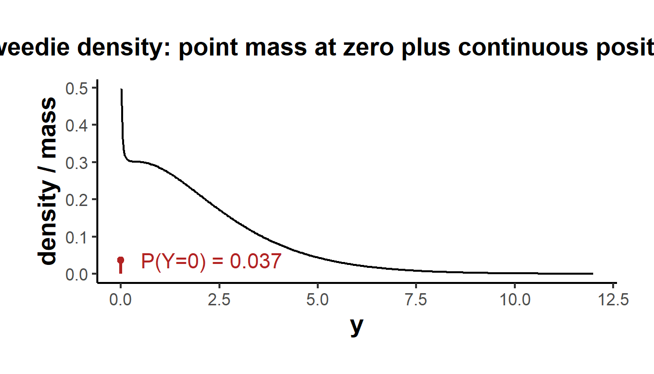

Figure 9.1: The Tweedie density for a mean of two, dispersion one, and power 1.6. A point mass sits at zero (here about four percent of the probability) and a continuous, right skewed density covers the positive values. No standard GLM distribution has this shape.

The variance function itself is the cleanest way to see where the Tweedie sits among its neighbors. Because \(\operatorname{Var}(Y) = \phi\,\mu^{p}\), the power \(p\) controls how fast the variance grows with the mean, interpolating continuously between the constant variance of the Gaussian, the linear variance of the Poisson, and the quadratic variance of the Gamma.

mu_seq <- seq(0.2, 5, length.out = 200)
vf <- do.call(rbind, lapply(
  c(`p=0 (Gaussian)` = 0, `p=1 (Poisson)` = 1, `p=1.5 (Tweedie)` = 1.5,
    `p=2 (Gamma)` = 2, `p=3 (inverse Gaussian)` = 3),
  function(p) data.frame(mu = mu_seq, V = mu_seq^p)
))
vf$power <- rep(c("p=0 (Gaussian)", "p=1 (Poisson)", "p=1.5 (Tweedie)",
                  "p=2 (Gamma)", "p=3 (inverse Gaussian)"), each = length(mu_seq))

ggplot(vf, aes(mu, V, colour = power)) +
  geom_line(linewidth = 0.8) +
  labs(x = expression(mu), y = expression(V(mu) == mu^p),
       colour = NULL, title = "Tweedie variance functions") +
  causalverse::ama_theme()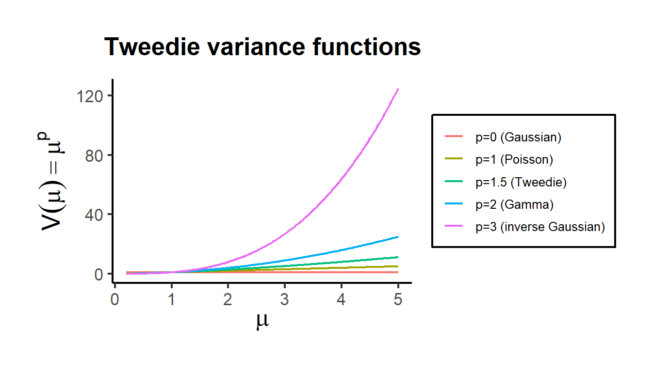

Figure 9.2: The Tweedie variance function for several powers of the mean. The power parameter interpolates continuously between the Gaussian (constant variance), the Poisson (linear), the Gamma (quadratic), and the inverse Gaussian (cubic).

9.4 Estimation: Mean, Dispersion, and Power

Fitting a Tweedie regression means estimating three things: the regression coefficients \(\beta\) in \(\log\mu_i = x_i^\top\beta\), the dispersion \(\phi\), and the power \(p\). They are estimated in a nested way that exploits a convenient fact: for any fixed \(p\), the coefficients are estimated by ordinary GLM machinery, and only the power requires anything special.

9.4.1 The Mean Model for Fixed Power

Hold \(p\) fixed. The Tweedie is then an ordinary exponential dispersion model with variance function \(V(\mu) = \mu^p\), and the coefficients are estimated by iteratively reweighted least squares, the same Fisher scoring algorithm that fits every GLM. The score equations for \(\beta\) are \[ \sum_{i=1}^{n} \frac{y_i - \mu_i}{\phi\, V(\mu_i)}\,\frac{\partial \mu_i}{\partial \eta_i}\, x_i = 0, \qquad \eta_i = x_i^\top\beta, \] which depend on the distribution only through the variance function \(V(\mu_i) = \mu_i^{p}\) and not through the intractable density. Each IRLS iteration regresses a working response on the covariates with working weights \[ w_i = \frac{1}{V(\mu_i)}\left(\frac{\partial \mu_i}{\partial \eta_i}\right)^{2} = \frac{\mu_i^{2}}{\mu_i^{p}} = \mu_i^{2-p} \] under the log link, and iterates to convergence. Because the score equations are exactly the quasi-likelihood estimating equations, the coefficient estimates are consistent as long as the mean model and the variance function are correct, even if the full Tweedie distribution is not literally true, which is one reason the model is so robust in practice. The deviance that IRLS minimizes is the sum of unit deviances \[ d(y, \mu) = 2\left[\frac{y\,(y^{1-p} - \mu^{1-p})}{1-p} - \frac{y^{2-p} - \mu^{2-p}}{2-p}\right], \qquad p \neq 1, 2, \] with the obvious limits recovering the Poisson and Gamma deviances at the endpoints. In R the variance function and link are supplied by the tweedie family from the statmod package, after which glm fits the model exactly as it would a Poisson or Gamma.

9.4.2 Estimating the Dispersion

Given the fitted means, the dispersion \(\phi\) is estimated either by the mean Pearson statistic, \(\hat\phi = \frac{1}{n-k}\sum_i (y_i - \hat\mu_i)^2 / \hat\mu_i^{p}\), or by maximum likelihood, which requires the density and is therefore a little more work but is what the likelihood based comparisons below rely on. The Pearson estimate is the GLM default and is what summary.glm reports as the dispersion.

9.4.3 Estimating the Power by Profile Likelihood

The power \(p\) is the one parameter that the GLM cannot estimate on its own, because it indexes which distribution we are fitting rather than a parameter within a fixed distribution. It is estimated by profile likelihood: for each candidate \(p\) on a grid, fit the GLM, estimate the dispersion, evaluate the full Tweedie log-likelihood at the fitted values using the density routines, and choose the \(p\) that maximizes it. This is the one step that genuinely needs the intractable density, which is why the whole apparatus of Dunn and Smyth (2005) and Dunn and Smyth (2008) exists. The profile is transparent enough to write directly: loop over \(p\), fit, and sum the log density. The simulation in the next section does exactly that and shows it recovers a known power.

9.5 A Simulation That Recovers the Truth

The cleanest way to confirm that the estimation works is to generate data from a known Tweedie model and recover its parameters. We draw a compound Poisson–Gamma response with a true power of \(1.6\), a log linear mean depending on one covariate, and a known dispersion, then profile the power by hand and fit the coefficients at the estimate.

library(statmod)
library(tweedie)

set.seed(2026)
n <- 3000
x  <- runif(n, -1, 1)
mu <- exp(1.5 + 0.8 * x)                 # true log-linear mean
y  <- rtweedie(n, mu = mu, phi = 2, power = 1.6)   # true phi = 2, p = 1.6

# Profile log-likelihood for the power: for each p, fit the GLM and sum the
# Tweedie log-density at the fitted mean and Pearson dispersion.
profile_power <- function(y, x, p_grid) {
  vapply(p_grid, function(p) {
    fit <- glm(y ~ x, family = tweedie(var.power = p, link.power = 0))
    sum(log(dtweedie(y, mu = fitted(fit),
                     phi = summary(fit)$dispersion, power = p)))
  }, numeric(1))
}

p_grid <- seq(1.3, 1.9, by = 0.05)
logL   <- profile_power(y, x, p_grid)
p_hat  <- p_grid[which.max(logL)]

ggplot(data.frame(p = p_grid, logL = logL), aes(p, logL)) +
  geom_line(linewidth = 0.8) +
  geom_vline(xintercept = 1.6, linetype = "dashed") +
  geom_point(data = data.frame(p = p_hat, logL = max(logL)),
             colour = "firebrick", size = 3) +
  labs(x = "power p", y = "profile log-likelihood",
       title = paste0("Profiled power = ", p_hat, " (truth 1.6)")) +
  causalverse::ama_theme()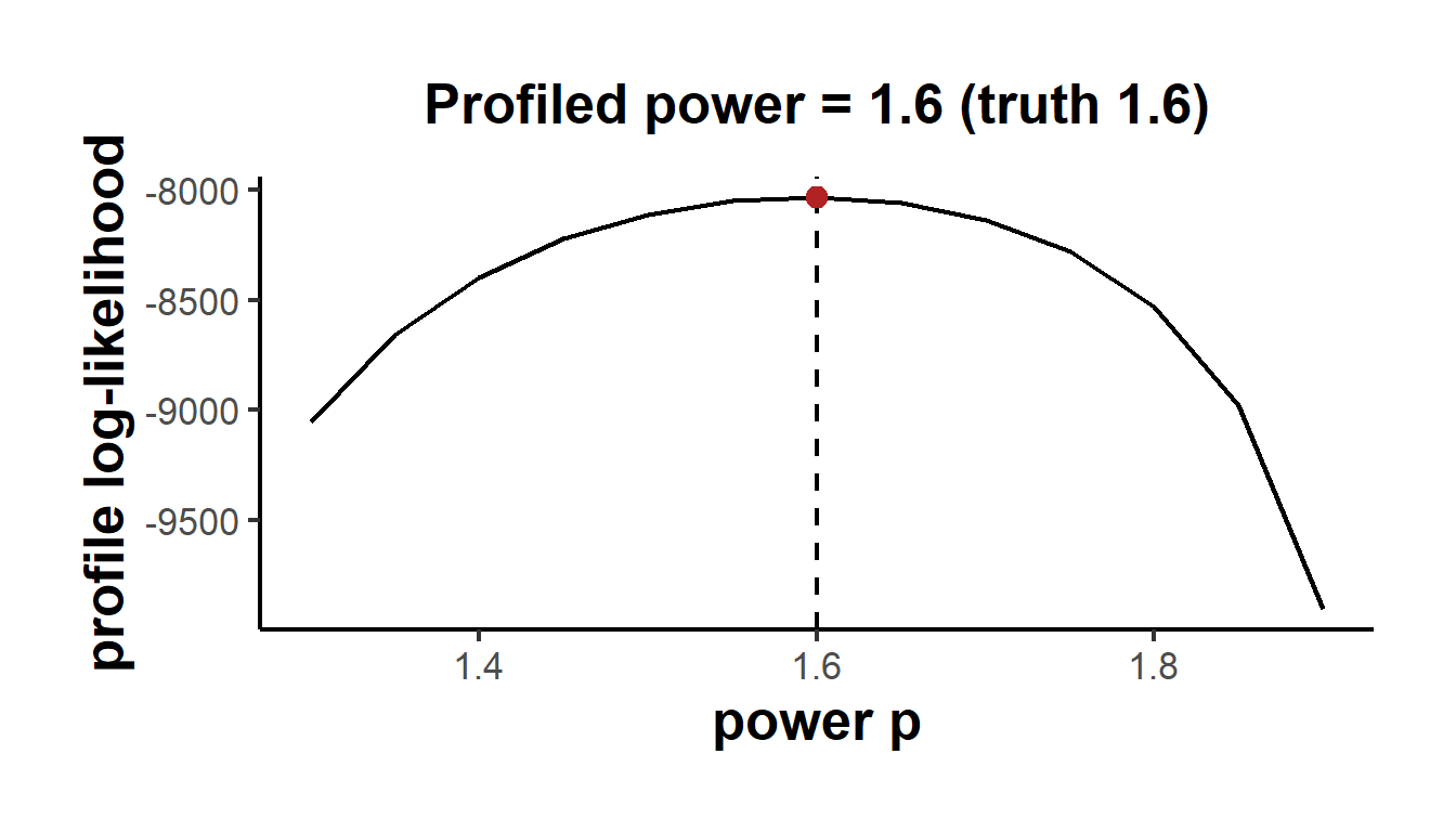

Figure 9.3: Profile log-likelihood for the Tweedie power parameter on simulated data whose true power is 1.6 (dashed line). The profile peaks at the truth, confirming that the power is identified and recovered.

fit_sim <- glm(y ~ x, family = tweedie(var.power = p_hat, link.power = 0))
knitr::kable(
  data.frame(
    Parameter = c("Intercept", "Slope (x)", "Dispersion phi", "Power p"),
    Truth = c(1.5, 0.8, 2.0, 1.6),
    Estimate = round(c(coef(fit_sim), summary(fit_sim)$dispersion, p_hat), 3)
  ),
  caption = "Tweedie regression recovers the data-generating parameters on simulated compound Poisson-Gamma data.",
  align = c("l", "r", "r")
)

Table 9.1: Tweedie regression recovers the data-generating parameters on simulated compound Poisson-Gamma data.

Parameter	Truth	Estimate
Intercept	1.5	1.506
Slope (x)	0.8	0.839
Dispersion phi	2.0	1.967
Power p	1.6	1.600

The profile peaks at the true power and the coefficients and dispersion land on their data generating values, confirming that the three part estimation scheme works as intended.

9.6 Real-Data Application: Insurance Pure Premium

Modeling insurance claim costs is the application that drove the development of the Tweedie GLM by Jørgensen and Souza (1994) and Smyth and Jørgensen (2002), and it remains the textbook use of the model. Those authors worked with their own proprietary portfolios, so rather than reproduce their exact numbers we apply the same method to a standard public benchmark, the dataCar portfolio distributed with the insuranceData package and analyzed at length in the insurance GLM textbook of de Jong and Heller (2008). It is a real Australian automobile insurance dataset of 67,856 one year policies. The response claimcst0 is the total claim cost incurred by each policy, and the covariates are the usual rating factors: the vehicle value and body type, the vehicle age, the driver’s age band and gender, and the geographic area. Each policy is observed for a known fraction of a year, the exposure, which enters the model as a weight so that the estimated mean is a rate per unit exposure, the pure premium. Because de Jong and Heller (2008) fit and interpret frequency and severity GLMs on exactly this data, their conclusions give us an external benchmark against which to check our own, which is the right way to read a replication: the test is whether the substantive findings agree, not merely whether the code runs.

library(insuranceData)
data(dataCar)

prop_zero <- mean(dataCar$claimcst0 == 0)

ggplot(subset(dataCar, claimcst0 > 0), aes(claimcst0)) +
  geom_histogram(bins = 50) +
  scale_x_continuous(labels = scales::dollar) +
  labs(x = "annual claim cost (positive policies)", y = "count",
       title = paste0("Claim cost: ", round(100 * prop_zero, 1),
                      "% of policies are exactly zero")) +
  causalverse::ama_theme()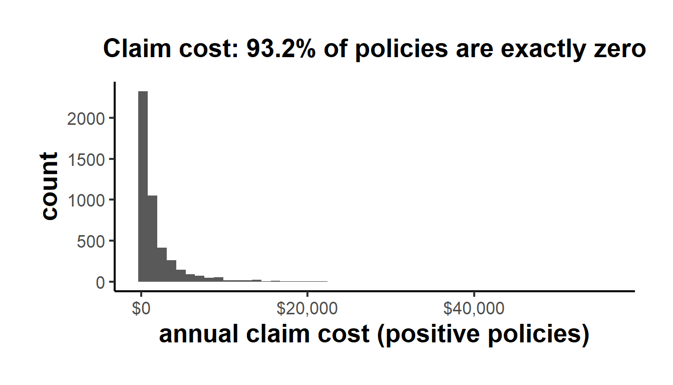

Figure 9.4: Distribution of annual claim cost in the dataCar portfolio. About 93 percent of policies cost zero (the bar at the origin), and the rest form a long right tail. This zero-inflated, continuous, right-skewed shape is the signature of a Tweedie response.

The modeling target is the pure premium, the expected cost per unit of exposure, so we form the response as cost divided by exposure and weight each observation by its exposure, the standard actuarial construction of Ohlsson and Johansson (2010). We first profile the power on a subsample, then fit the Tweedie GLM at the chosen power on the full portfolio.

library(statmod)
library(tweedie)

d <- dataCar
d$agecat  <- factor(d$agecat)
d$veh_age <- factor(d$veh_age)
d$pp <- d$claimcst0 / d$exposure          # pure premium response
form <- pp ~ veh_body + veh_age + agecat + gender + area

# Profile the power on a subsample (the density evaluation is the costly step).
set.seed(1)
sub <- d[sample(nrow(d), 12000), ]
p_grid <- seq(1.4, 1.7, by = 0.05)
logL <- vapply(p_grid, function(p) {
  f <- glm(form, data = sub, weights = exposure,
           family = tweedie(var.power = p, link.power = 0))
  sum(log(dtweedie(sub$pp, mu = fitted(f),
                   phi = summary(f)$dispersion, power = p)))
}, numeric(1))
p_hat <- p_grid[which.max(logL)]
p_hat
#> [1] 1.7

The likelihood favors a power near \(1.7\), within the range of roughly \(1.5\) to \(1.8\) typically reported for automobile claim costs and consistent with a portfolio in which most policies have no claim and the positive costs are heavily skewed. The value sits a little above the estimate that the smooth mgcv fit returns later in the chapter, a reminder that the power estimate moves with the mean specification and the estimation method. With the power fixed, the coefficients are an ordinary GLM fit, and because of the log link each exponentiated coefficient is a multiplicative relativity, the factor by which a rating cell scales the baseline pure premium.

fit <- glm(form, data = d, weights = exposure,
           family = tweedie(var.power = p_hat, link.power = 0))

co <- summary(fit)$coefficients
keep <- grep("agecat|genderM", rownames(co))
knitr::kable(
  data.frame(
    Factor = rownames(co)[keep],
    Relativity = round(exp(co[keep, "Estimate"]), 3),
    `Std. Error (log)` = round(co[keep, "Std. Error"], 3),
    `p-value` = round(co[keep, "Pr(>|t|)"], 3),
    check.names = FALSE
  ),
  row.names = FALSE,
  caption = "Pure-premium relativities for driver age band and gender from the Tweedie GLM on the dataCar portfolio (baseline: youngest age band, female). A relativity below one means cheaper than baseline. The standard error and p-value are on the log (coefficient) scale. The age-band effects are strongly significant; the gender effect is not.",
  align = c("l", "r", "r", "r")
)

Table 9.2: Pure-premium relativities for driver age band and gender from the Tweedie GLM on the dataCar portfolio (baseline: youngest age band, female). A relativity below one means cheaper than baseline. The standard error and p-value are on the log (coefficient) scale. The age-band effects are strongly significant; the gender effect is not.

Factor	Relativity	Std. Error (log)	p-value
agecat2	0.692	0.238	0.122
agecat3	0.599	0.232	0.027
agecat4	0.590	0.231	0.022
agecat5	0.430	0.251	0.001
agecat6	0.470	0.283	0.007
genderM	1.151	0.127	0.266

The relativities tell a clear and, importantly, externally corroborated story. The age bands run from one, the youngest drivers, to six, the oldest, and the youngest band is the most expensive: every older band has a relativity below one, the cost of insuring a policy falling from the young baseline to roughly forty three percent for the second oldest band before ticking back up slightly for the very oldest, the mild U shape that actuaries expect when both inexperienced young drivers and the very old are riskier than those in between. Four of the five age coefficients are significant at conventional levels, so this pattern is real. The gender relativity is a different matter and is where reading the table honestly matters. The point estimate suggests male policies cost about fifteen percent more, but its p value is roughly \(0.27\), so the effect is not statistically distinguishable from zero once the other rating factors are controlled for. This is exactly what de Jong and Heller (2008) find on the same data, that gender carries little signal for this portfolio, and it is a useful caution against reading a rate relativity off a point estimate without checking whether the data support it. Age belongs in the rating table; gender, on this evidence, does not.

A first check on any pure premium model is whether it reproduces the total cost of the portfolio, since a model used to set prices must at least get the aggregate right. The Tweedie GLM with a log link has this calibration built in through its score equations.

predicted_total <- sum(fitted(fit) * d$exposure)
actual_total    <- sum(d$claimcst0)
knitr::kable(
  data.frame(
    Quantity = c("Predicted total cost", "Actual total cost", "Ratio"),
    Value = c(scales::dollar(predicted_total), scales::dollar(actual_total),
              round(predicted_total / actual_total, 4))
  ),
  caption = "The Tweedie pure-premium model reproduces the aggregate claim cost of the portfolio almost exactly, a basic requirement for a pricing model.",
  align = c("l", "r")
)

Table 9.3: The Tweedie pure-premium model reproduces the aggregate claim cost of the portfolio almost exactly, a basic requirement for a pricing model.

Quantity	Value
Predicted total cost	$9,309,027
Actual total cost	$9,314,604
Ratio	0.9994

9.6.1 Comparison With the Two-Part Frequency–Severity Model

The traditional actuarial alternative to the Tweedie splits the problem in two: a frequency model for the number of claims and a severity model for the average cost per claim, multiplied together to give the pure premium. The frequency is a Poisson (or negative binomial) GLM with an exposure offset, and the severity is a Gamma GLM fit on the policies that did claim. The Tweedie is, in a precise sense, the single distribution that fuses these two stages, which is why its power parameter encodes the frequency–severity split. Fitting both lets us compare them on the same portfolio.

# Frequency: Poisson claim count with a log-exposure offset.
freq <- glm(numclaims ~ veh_body + veh_age + agecat + gender + area,
            offset = log(exposure), family = poisson, data = d)
# Severity: Gamma average cost per claim, on policies with at least one claim.
pos  <- subset(d, claimcst0 > 0)
sev  <- glm(claimcst0 / numclaims ~ veh_body + veh_age + agecat + gender + area,
            weights = numclaims, family = Gamma(link = "log"), data = pos)

twopart_total <- sum(predict(freq, type = "response") *
                     predict(sev, newdata = d, type = "response"))
knitr::kable(
  data.frame(
    Model = c("Tweedie (single GLM)", "Frequency x Severity (two GLMs)", "Actual"),
    `Predicted total cost` = c(scales::dollar(predicted_total),
                               scales::dollar(twopart_total),
                               scales::dollar(actual_total)),
    check.names = FALSE
  ),
  row.names = FALSE,
  caption = "The Tweedie GLM and the classical two-part frequency-severity model give very similar aggregate predictions. The Tweedie achieves this with a single model and a single set of coefficients rather than two.",
  align = c("l", "r")
)

Table 9.4: The Tweedie GLM and the classical two-part frequency-severity model give very similar aggregate predictions. The Tweedie achieves this with a single model and a single set of coefficients rather than two.

Model	Predicted total cost
Tweedie (single GLM)	$9,309,027
Frequency x Severity (two GLMs)	$9,315,807
Actual	$9,314,604

The two approaches land in the same place on the aggregate, which is reassuring, but the Tweedie does it with one model rather than two, one set of coefficients to interpret rather than two, and without the awkwardness of the severity model being undefined for the ninety three percent of policies that never claim. The cost is that the Tweedie blends frequency and severity effects into a single coefficient, so when an analyst specifically wants to know whether a factor drives how often people claim or how much they claim, the two part model remains more informative. The choice between them is a choice about what question is being asked, not about which is correct.

9.7 Beyond the GLM: Smooth, Regularized, and Boosted Tweedie Models

The Tweedie response is not tied to the linear predictor of a GLM; it is a likelihood that can sit on top of any modern regression engine, and the same actuarial and scientific problems that motivate it have driven its incorporation into flexible models.

A Tweedie generalized additive model replaces linear terms with smooth functions, which is valuable when a rating factor such as vehicle value or driver age has a nonlinear effect on cost. The mgcv package fits these and, unlike the GLM workflow above, estimates the power parameter jointly with the smooths by restricted maximum likelihood, so the analyst does not profile it by hand.

library(mgcv)
gam_fit <- gam(pp ~ s(veh_value) + veh_body + agecat + gender,
               weights = exposure, family = tw(), data = d, method = "REML")
cat("mgcv estimated Tweedie power p =",
    round(gam_fit$family$getTheta(TRUE), 3), "\n")
#> mgcv estimated Tweedie power p = 1.606

The REML estimate of the power, near \(1.6\), sits a little below the GLM profile estimate, a reminder that the power is estimated jointly with the rest of the model and shifts with the mean specification. For high-dimensional rating problems with many correlated factors, Qian et al. (2016) develop a grouped elastic net for the Tweedie compound Poisson model, implemented in the HDtweedie package, which selects and shrinks coefficients while respecting the grouping of a categorical factor’s dummy variables. For the flexible, interaction-rich models that dominate contemporary insurance practice, the Tweedie deviance is available as a loss function in gradient boosting libraries, so a boosted-tree pure premium model is a direct nonparametric extension of the GLM. Both are shown for reference rather than run, since they require additional packages and tuning.

# High-dimensional grouped elastic net (Qian, Yang & Zou 2016).
library(HDtweedie)
cv <- cv.HDtweedie(x = X, y = y, group = grp, p = 1.5)

# Gradient-boosted trees with the Tweedie deviance loss.
library(xgboost)
bst <- xgboost(data = X, label = y, nrounds = 200,
               objective = "reg:tweedie",
               tweedie_variance_power = 1.5)

A fully Bayesian and mixed-model treatment is available as well: Zhang (2013) develops likelihood-based and Bayesian estimation for Tweedie compound Poisson linear mixed models in the cplm package, which adds random effects to the structure above, the natural tool when policies are grouped within regions, agents, or years.

9.8 Practical Guidance and Pitfalls

A few points govern whether a Tweedie analysis goes smoothly.

The power parameter should be estimated, not assumed, but it need not be estimated precisely. The fit and the coefficients are fairly insensitive to small changes in \(p\) across the plausible range, so a profile on a coarse grid, or the REML estimate from mgcv, is usually enough. Fixing \(p\) at a round value such as \(1.5\) for a first pass is a reasonable habit, but the final model should report a profiled or jointly estimated power.

The exposure belongs in the model as a weight on the pure premium response, not as a covariate. Treating exposure as a regressor confounds the amount of time at risk with the rating factors and produces uninterpretable coefficients. The construction used above, response equal to cost over exposure with weights equal to exposure, is the standard one and makes the fitted mean a rate.

The numerical evaluation of the density can fail in the heavy tail. For very large responses, both the series and the inversion methods can return non-finite values, which is why the power profile above was restricted to a grid where the likelihood was computable and why the maximum sat at the edge of that grid rather than at a clean interior peak. When this happens, profiling on a subsample, trimming or capping a handful of extreme observations for the power estimation step only, or relying on the mgcv REML estimate are all reasonable responses; none of them affects the coefficient estimates, which never touch the density.

Finally, the Tweedie is a model of a mean, and like every GLM it identifies an association that is causal only under the usual assumptions. Its value is that it gets the distributional shape of a zero-inflated continuous response right, which makes its standard errors and predictions trustworthy where a Gaussian or log-normal model would not be, but it does not by itself license a causal reading of the rating factors. For pricing that is exactly what is wanted, since the goal is an accurate conditional mean rather than a counterfactual; for an application where a factor is meant to be a treatment, the identification has to come from the design, as everywhere else in this book.

📖 Free preview — limited per publisher guidelines. Purchase the complete A Guide on Data Analysis series (Vols. 1–4) on Springer.

Vol. 1 Vol. 2 Vol. 3 Vol. 4