64.1 Why Auctions Are a Canonical Structural Setting

Consider a single indivisible object sold to one of \(n\) bidders. Bidder \(i\) holds a valuation \(v_i\), a private number measuring willingness to pay, drawn from a distribution \(F\) with density \(f\) on a support \([\underline{v}, \overline{v}]\). The analyst observes the bids \(b_i\) that bidders submit but not the valuations \(v_i\) that generated them. In equilibrium each bidder follows a strategy \(b_i = \beta(v_i)\), a function that the theory pins down given the format and the informational environment. Because \(\beta\) is strictly increasing under standard conditions, it can be inverted, so that \(v_i = \beta^{-1}(b_i)\). The distribution of bids \(G\) and the distribution of valuations \(F\) are then linked by the change of variables

\[ G(b) = F\big(\beta^{-1}(b)\big), \]

and the structural task is to use the observed \(G\), together with the equilibrium restriction that fixes \(\beta\), to back out the unobserved \(F\). The power of the approach is that \(F\) is a primitive: it does not change when the auction format or the reserve price changes, so once recovered it supports counterfactuals about designs that were never run. This is the structural payoff that a purely descriptive model of bids cannot deliver.

64.2 Formats and Paradigms

The four classic single-object formats divide into two pairs. In the first-price sealed-bid auction each bidder submits one sealed bid and the highest bidder wins and pays the bid. In the Dutch auction a price descends from a high level until a bidder accepts, which is strategically equivalent to the first-price auction because the only decision is the price at which to commit. In the second-price sealed-bid auction, the Vickrey auction, the highest bidder wins but pays the second highest bid, and in the ascending English auction the price rises until one bidder remains. The second-price and English formats share the feature that, under private values, bidding one’s own valuation is a dominant strategy, so bids reveal valuations directly and the inversion problem is trivial. The first-price and Dutch formats shade bids below valuations by an amount that depends on competition and on beliefs about rivals, which is what makes their structural analysis interesting.

The informational paradigm matters as much as the format. Under independent private values (IPV), each bidder knows her own valuation, valuations are independent draws from \(F\), and one bidder’s valuation carries no information about another’s. Under the common value paradigm the object is worth the same unknown amount to all bidders, for example the recoverable oil under a tract, and each bidder sees only a private signal correlated with that common value. The intermediate and most general case is the affiliated values model of Milgrom and Weber (1982), in which valuations or signals are positively dependent, so that a high signal for one bidder makes high signals for others more likely. Affiliation nests both private and common values and delivers the central comparative result that, on average, the English auction raises more revenue than the second-price auction, which in turn raises more than the first-price auction, a ranking that collapses to revenue equivalence only in the independent private values benchmark.

The common value paradigm introduces the winner’s curse. The bidder who wins is the one whose signal was most optimistic, so conditioning on winning is bad news about the true value: the winner is precisely the bidder most likely to have overestimated. Rational bidders anticipate this and shade their bids to correct for the adverse selection inherent in winning. A bidder who bids naively, as if her signal were unbiased even conditional on winning, will systematically overpay. The winner’s curse is not a behavioral mistake in the equilibrium model but a force that disciplined bidders build into their strategies, and detecting whether bidders account for it is one empirical reason to distinguish common from private values.

64.3 Identification and Estimation

64.4 Extensions

The baseline estimator extends in several directions that matter for applied work. Risk aversion breaks the neutral first-order condition above, because a risk averse bidder values the certainty of winning more and therefore bids more aggressively; the same observed bids are then consistent with a different and less dispersed valuation distribution, so risk attitudes and valuation heterogeneity are entangled and require either functional form restrictions or exclusion variation to separate. Unobserved heterogeneity across auctions, where some auctions attract systematically higher or lower valuations for reasons the analyst does not record, contaminates the pooled bid distribution and biases the naive inversion. Krasnokutskaya (2011) showed how to identify and strip out such auction level unobserved heterogeneity using deconvolution, exploiting the multiplicative or additive separability of the unobserved component from the idiosyncratic bidder draw. Entry introduces a prior stage in which potential bidders decide whether to incur a cost to participate, so the set of actual bidders is selected and the number of bidders is endogenous, which must be modeled jointly with the bidding stage to avoid confounding selection with valuation differences. Finally, testing private versus common values uses the comparative statics of bids in the number of competitors, since adding rivals intensifies the winner’s curse correction under common values but only the competition effect under private values, giving a testable distinction grounded in the identification difficulties noted above.

64.5 Policy and Counterfactual Design

The reason to recover \(F\) rather than merely describe bids is that \(F\) supports counterfactual reasoning about designs the seller might choose. The leading application is the optimal reserve price. A reserve price excludes low valuations and so risks losing a sale, but it also forces bidders above the reserve to compete against a credible outside option, raising the price they pay. Knowledge of \(F\) lets the analyst compute the reserve that maximizes expected revenue, which under regularity is the value \(r\) solving \(r - (1 - F(r))/f(r) = v_0\), where \(v_0\) is the seller’s own valuation, exactly the marginal revenue logic of monopoly pricing applied to the bidder with the reserve valuation. Revenue comparisons across formats follow the same template: with \(F\) in hand the analyst simulates the first-price, second-price, and ascending formats and reports which raises more, recovering the revenue equivalence benchmark under IPV and the affiliation-driven ranking otherwise. More broadly, the recovered primitive underwrites counterfactual mechanism design, evaluating bidder subsidies, set-asides, reserve schedules, and entry promotion against the revenue and efficiency they would deliver, none of which is answerable from observed bids alone because each counterfactual changes the equilibrium bidding strategy and hence the bid distribution itself.

64.6 Simulation: Estimating Valuations from First-Price Bids

To make the inversion concrete we simulate a symmetric IPV first-price auction in which valuations are uniform on the unit interval, a case for which the equilibrium bid function has the closed form \(\beta(v) = v\,(n-1)/n\). We draw valuations, compute equilibrium bids from this closed form, and then pretend we observe only the bids. Applying the Guerre et al. (2000) inversion, we estimate the bid distribution by its empirical CDF and the bid density by a kernel, recover a pseudo-value for each bid through the first-order condition, and compare the distribution of recovered values against the known truth.

# Symmetric IPV first-price auction with Uniform(0,1) valuations.
# Equilibrium bid function: beta(v) = v * (n - 1) / n.
n_bidders <- 5          # bidders per auction
n_auctions <- 4000      # number of independent auctions

# Draw one representative bidder's valuation per auction, then all bids.
# For the inversion we pool bids across auctions (same n in each).
v_true <- runif(n_auctions * n_bidders)          # latent valuations
b_obs  <- v_true * (n_bidders - 1) / n_bidders    # equilibrium bids

# Step 1: nonparametric estimates of the bid CDF and bid density.
G_hat <- ecdf(b_obs)                              # empirical bid CDF
dens  <- density(b_obs, n = 1024)                 # kernel bid density
g_hat <- approxfun(dens$x, dens$y, rule = 2)      # interpolate density

# Step 2: GPV inversion. Each bid maps to a pseudo-value via the FOC:
#   v = b + (1 / (n - 1)) * G(b) / g(b).
v_hat <- b_obs + (1 / (n_bidders - 1)) * G_hat(b_obs) / g_hat(b_obs)

# Trim a small fraction near the boundaries where the kernel density is
# unreliable, a standard precaution with the GPV estimator.
keep  <- b_obs > quantile(b_obs, 0.02) &
         b_obs < quantile(b_obs, 0.98)
v_hat_trim  <- v_hat[keep]
v_true_trim <- v_true[keep]

The pseudo-values in v_hat are the recovered valuations. Because the data generating process is known, we can check the recovery directly. The table below compares quantiles of the true valuation distribution against quantiles of the recovered one, and the figure overlays the two densities.

probs <- c(0.10, 0.25, 0.50, 0.75, 0.90)
auc_tab <- data.frame(
  Quantile        = probs,
  Value_true      = round(quantile(v_true_trim, probs), 3),
  Value_recovered = round(quantile(v_hat_trim,  probs), 3)
)
auc_tab
#>     Quantile Value_true Value_recovered
#> 10%     0.10      0.114           0.115
#> 25%     0.25      0.262           0.262
#> 50%     0.50      0.502           0.499
#> 75%     0.75      0.737           0.737
#> 90%     0.90      0.883           0.887

The recovered quantiles sit close to the truth across the distribution. Figure 64.1 overlays the true and recovered valuation densities, confirming that the inversion recovers the latent valuations from bids alone without ever using the true valuations in the estimation. The agreement is not mechanical: the estimator saw only b_obs and the assumed equilibrium structure.

library(ggplot2)

plot_df <- rbind(
  data.frame(value = v_true_trim, series = "True valuations"),
  data.frame(value = v_hat_trim,  series = "Recovered (GPV)")
)

ggplot(plot_df, aes(value, color = series, fill = series)) +
  geom_density(alpha = 0.15, linewidth = 0.9) +
  labs(
    x = "Valuation",
    y = "Density",
    color = NULL, fill = NULL
  ) +
  causalverse::ama_theme()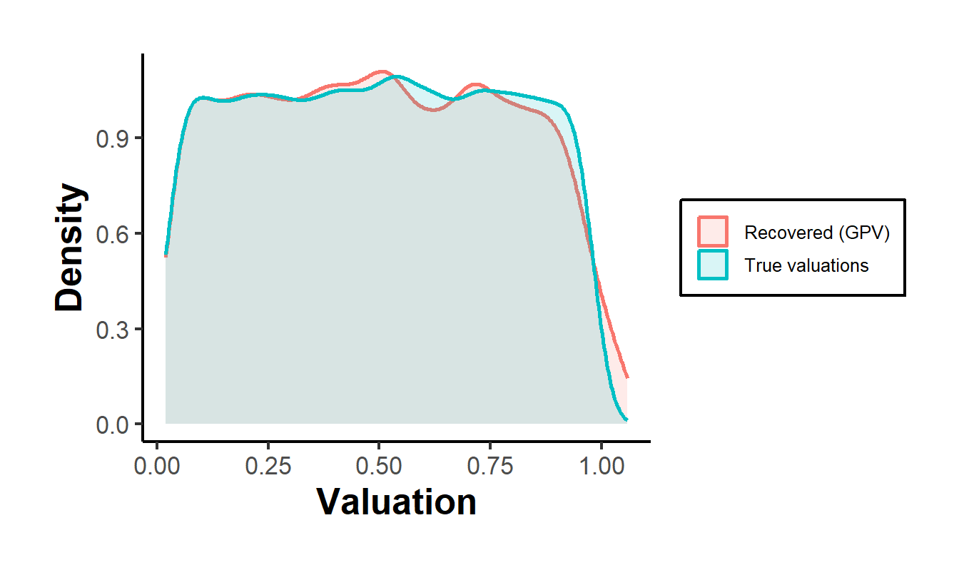

Figure 64.1: True versus recovered valuation densities for a symmetric IPV first-price auction with five bidders and Uniform(0,1) valuations. The recovered density is constructed by the Guerre, Perrigne, and Vuong inversion applied to observed bids only, with no use of the latent valuations.

The two densities are nearly coincident over the interior of the support, with the familiar boundary degradation that motivates the trimming: the kernel density of bids is biased near the edges of its support, which inflates the markup term \(G(b)/g(b)\) there and distorts the recovered values at the extreme quantiles. The exercise is a self-contained demonstration of the structural logic of the chapter. The auction rules supplied the first-order condition, the first-order condition supplied the inversion, and the inversion turned a distribution of observed bids into the distribution of unobserved valuations that the seller would need to choose a reserve price or compare formats.

64.7 Summary

Auctions are the cleanest illustration of the structural method because the equilibrium bid function is a known and invertible map from unobserved valuations to observed bids. The format fixes the strategic problem, the informational paradigm fixes the dependence structure, and together they determine whether bids reveal valuations directly, as in the second-price and English auctions under private values, or shade them in a way that must be undone, as in the first-price and Dutch auctions. The Guerre et al. (2000) two-step estimator performs that undoing nonparametrically by reading valuations off bids through the first-order condition, an inversion licensed by the identification results of Athey and Haile (2002) for private values and complicated, in the common value case, by the observational equivalence noted by Laffont et al. (1995). Extensions for risk aversion, unobserved heterogeneity in the manner of Krasnokutskaya (2011), and endogenous entry adapt the method to the messiness of field data, and the recovered valuation distribution is what makes optimal reserve prices, revenue comparisons, and counterfactual mechanism design tractable. The next chapters in the cluster carry the same recover-the-primitive logic into other equilibrium settings.