39 Instrumental Variables
In many empirical settings, we seek to estimate the causal effect of an explanatory variable \(X\) on an outcome variable \(Y\). A common starting point is the Ordinary Least Squares regression:
\[ Y = \beta_0 + \beta_1 X + \varepsilon. \]
For OLS to provide an unbiased and consistent estimate of \(\beta_1\), the explanatory variable \(X\) must satisfy the exogeneity condition:
\[ \mathbb{E}[\varepsilon \mid X] = 0. \]
However, when \(X\) is correlated with the error term \(\varepsilon\), this assumption is violated, leading to endogeneity. As a result, the OLS estimator is biased and inconsistent. Common causes of endogeneity include:
- Omitted Variable Bias (OVB): When a relevant variable is omitted from the regression, leading to correlation between \(X\) and \(\varepsilon\).
- Simultaneity: When \(X\) and \(Y\) are jointly determined, such as in supply-and-demand models.
- Measurement Error: Errors in measuring \(X\) introduce bias in estimation.
- Attenuation Bias in Errors-in-Variables: measurement error in the independent variable leads to an underestimate of the true effect (biasing the coefficient toward zero).
Instrumental Variables (IV) estimation addresses endogeneity by introducing an instrument \(Z\) that affects \(Y\) only through \(X\). Similar to RCT, we try to introduce randomization (random assignment to treatment) to our treatment variable by using only variation in the instrument.
Logic of using an instrument:
Use only exogenous variation to see the variation in treatment (try to exclude all endogenous variation in the treatment)
Use only exogenous variation to see the variation in outcome (try to exclude all endogenous variation in the outcome)
See the relationship between treatment and outcome in terms of residual variations that are exogenous to omitted variables.
For an instrument \(Z\) to be valid, it must satisfy two conditions:
Relevance Condition: The instrument \(Z\) must be correlated with the endogenous variable \(X\): \[ \text{Cov}(Z, X) \neq 0. \]
Exogeneity Condition (Exclusion Restriction): The instrument \(Z\) must be uncorrelated with the error term \(\varepsilon\) and affect \(Y\) only through \(X\): \[ \text{Cov}(Z, \varepsilon) = 0. \]
These conditions ensure that \(Z\) provides exogenous variation in \(X\), allowing us to isolate the causal effect of \(X\) on \(Y\).
These conditions ensure that \(Z\) provides exogenous variation in \(X\), allowing us to estimate the causal effect of \(X\) on \(Y\). Random assignment of \(Z\) helps ensure exogeneity, but we must also confirm that \(Z\) influences \(Y\) only through \(X\) to satisfy the exclusion restriction.
A note on weak instruments before we go further. Relevance is a quantitative requirement, not a binary one: a statistically significant first stage is not sufficient evidence that the instrument is strong enough. Even a mildly weak instrument can produce 2SLS estimates that are severely biased toward OLS, with confidence intervals that undercover dramatically in finite samples.
The conventional rules of thumb you will encounter later in this chapter are:
- A first-stage F-statistic below 10 (the Staiger-Stock threshold) indicates a weak instrument and unreliable 2SLS estimates.
- F-statistics between 10 and 20 were historically considered adequate, but Lee et al. (2022) show the conventional critical values are too permissive in this range. Weak-instrument-robust inference (Anderson-Rubin, CLR) is preferable to reading the 2SLS t-statistic directly.
- F-statistics above 20 are a safer threshold under modern guidance.
- With multiple instruments (overidentified models), use the Montiel Olea-Pflueger effective F-statistic rather than the standard first-stage F. See the weak-instruments section later in this chapter for implementation details.
One point is worth internalizing now: weak-instrument bias does not vanish with larger sample sizes. It is a property of first-stage strength, not of sampling noise. When the instrument is weak, the remedies are weak-instrument-robust methods (Anderson-Rubin, LIML, CLR) or partial identification bounds, not a larger \(N\).
It is worth a brief detour through the history, because the trajectory of the IV idea explains a great deal about how the method is used today. The technique dates back to early econometric work in the 1920s and 1930s, when researchers grappling with simultaneous-equations models needed a way to disentangle systems in which prices and quantities, or any pair of jointly determined variables, were chasing each other. One of the earliest applications was Wright (1928)’s study of supply and demand for pig iron, an exemplar that would resurface a generation later in the Cowles Commission programme on identification. For decades thereafter IV remained a specialist’s tool, used mostly in macroeconomics and demand estimation.
The method’s modern centrality dates from the credibility revolution of the 1990s and 2000s, which reframed identification as a research-design problem rather than a modelling one. Angrist and Imbens (1991)’s use of quarter-of-birth as an instrument for years of schooling is the canonical example: a clever, almost incidental source of variation that arguably has no business affecting earnings except through its effect on education. That paper, along with a wave of similar designs, repositioned IV as a workhorse for applied research in economics, political science, and epidemiology, wherever a credible exogenous shock to the variable of interest could be located in nature, in policy, or in institutional accident.
39.1 Challenges with Instrumental Variables
While IVs can provide a solution to endogeneity, the practical difficulties cluster into three families: assumption failures (an exclusion restriction that does not actually hold, or an instrument that is too weak to identify anything reliably), interpretation traps (the LATE applies only to compliers, not to the population the reader probably has in mind), and design hygiene (the same instrument used many times across literatures eventually becomes implausible). In any given application, the exclusion restriction and weak-instrument concerns are usually the ones that decide whether the analysis is publishable, but each of the points below has historically been the issue that broke a published result.
Exclusion-restriction violations. If the instrument \(Z\) affects \(Y\) through any channel other than \(X\), the IV estimate is biased. The bias is not signed in general: a backdoor channel that pushes \(Y\) in the same direction as the treatment makes IV overstate the effect, while a channel that pushes the other way makes IV understate it. The exclusion restriction is fundamentally untestable, so the discipline here is to argue it explicitly from institutional knowledge and to probe it with falsification tests on placebo outcomes.
Repeated use of instruments. Common instruments such as weather, distance to a regulator, or sweeping policy changes can be invalidated by their widespread application across studies (Gallen 2020): an instrument that has been shown to predict many outcomes is one that almost certainly violates the exclusion restriction for at least some of them. The canonical illustration is Mellon (2021), who documents that 289 social-science studies have used weather as an instrument for 195 distinct variables, an aggregate pattern that is hard to reconcile with the exclusion restriction holding for any single application. The defensive moves are to argue for the exclusion in your specific setting rather than relying on the literature’s collective use of the instrument, to use formal tests for invalid instruments (Hausman-like tests, overidentification tests, the Conley-Hansen-Rossi plausibly exogenous bounds), and to run sensitivity analyses across the modest violations of exclusion that the most plausible alternative channels would imply.
Heterogeneous treatment effects and the LATE. The Local Average Treatment Effect estimated by IV applies only to compliers: units whose treatment status is shifted by the instrument. The complier subpopulation is rarely the one a policymaker has in mind, and it is unobservable to the analyst, so the estimate corresponds to a weighted average of unit-level effects with weights the analyst cannot directly inspect. When the treatment effect is constant across units, the LATE coincides with the ATE and the distinction does not matter; when effects are heterogeneous, the LATE can be substantively different from the ATE, and reporting the LATE without flagging the distinction misleads readers.
Weak instruments. Insufficient correlation between the instrument and the endogenous regressor produces unstable 2SLS estimates with confidence intervals that undercover the truth in finite samples. The standard test is the first-stage F-statistic, with thresholds discussed at length in the weak-instruments section later in this chapter; the standard remedies are weak-instrument-robust methods (Anderson-Rubin, CLR, LIML) or partial-identification approaches when robust inference is too imprecise to be useful.
Invalid instruments more broadly. Even when the first stage is strong and the instrument has not been used elsewhere, it can fail the exogeneity assumption for institution-specific reasons that the analyst missed. The best safeguard is a careful institutional argument paired with placebo and balance tests: an instrument that predicts pre-treatment outcomes or covariates that should be unaffected by it is an instrument that has not survived scrutiny.
Interpretation mistakes. Even when everything else is correct, the IV result identifies only the effect for the marginal units whose treatment status is shifted by the instrument. A policy that rolls out a treatment to a different subpopulation will not, in general, have the LATE-implied effect. Reporting the estimand explicitly, distinguishing it from the ATE and from the ATT, and discussing the share of compliers in the sample are the disciplines that keep the interpretation honest.
39.2 Framework for Instrumental Variables
We consider a binary treatment framework where:
\(D_i \sim Bernoulli(p)\) is a dummy treatment variable.
\((Y_{0i}, Y_{1i})\) are the potential outcomes under control and treatment.
The observed outcome is: \[ Y_i = Y_{0i} + (Y_{1i} - Y_{0i}) D_i. \]
-
We introduce an instrumental variable \(Z_i\) satisfying: \[ Z_i \perp (Y_{0i}, Y_{1i}, D_{0i}, D_{1i}). \]
- This means \(Z_i\) is independent of potential outcomes and potential treatment status.
- \(Z_i\) must also be correlated with \(D_i\) to satisfy the relevance condition.
39.2.1 Constant-Treatment-Effect Model
Under the constant treatment effect assumption (i.e., the treatment effect is the same for all individuals),
\[ \begin{aligned} Y_{0i} &= \alpha + \eta_i, \\ Y_{1i} - Y_{0i} &= \rho, \\ Y_i &= Y_{0i} + D_i (Y_{1i} - Y_{0i}) \\ &= \alpha + \eta_i + D_i \rho \\ &= \alpha + \rho D_i + \eta_i. \end{aligned} \]
where:
- \(\eta_i\) captures individual-level heterogeneity.
- \(\rho\) is the constant treatment effect.
The problem with OLS estimation is that \(D_i\) may be correlated with \(\eta_i\), leading to endogeneity bias.
39.2.2 Instrumental Variable Solution
A valid instrument \(Z_i\) allows us to estimate the causal effect \(\rho\) via:
\[ \begin{aligned} \rho &= \frac{\text{Cov}(Y_i, Z_i)}{\text{Cov}(D_i, Z_i)} \\ &= \frac{\text{Cov}(Y_i, Z_i) / V(Z_i) }{\text{Cov}(D_i, Z_i) / V(Z_i)} \\ &= \frac{\text{Reduced form estimate}}{\text{First-stage estimate}} \\ &= \frac{E[Y_i |Z_i = 1] - E[Y_i | Z_i = 0]}{E[D_i |Z_i = 1] - E[D_i | Z_i = 0 ]}. \end{aligned} \]
This ratio measures the treatment effect only if \(Z_i\) is a valid instrument.
39.2.3 Heterogeneous Treatment Effects and the LATE Framework
In a more general framework where treatment effects vary across individuals,
Define potential outcomes as: \[ Y_i(d,z) = \text{outcome for unit } i \text{ given } D_i = d, Z_i = z. \]
-
Define treatment status based on \(Z_i\): \[ D_i = D_{0i} + Z_i (D_{1i} - D_{0i}). \]
where:
- \(D_{1i}\) is the treatment status when \(Z_i = 1\).
- \(D_{0i}\) is the treatment status when \(Z_i = 0\).
- \(D_{1i} - D_{0i}\) is the causal effect of \(Z_i\) on \(D_i\).
39.2.4 Assumptions for LATE Identification
39.2.4.1 Independence (Instrument Randomization)
The instrument must be as good as randomly assigned:
\[ [\{Y_i(d,z); \forall d, z \}, D_{1i}, D_{0i} ] \perp Z_i. \]
This ensures that \(Z_i\) is uncorrelated with potential outcomes and potential treatment status.
This assumption let the first-stage equation be the average causal effect of \(Z_i\) on \(D_i\)
\[ \begin{aligned} E[D_i |Z_i = 1] - E[D_i | Z_i = 0] &= E[D_{1i} |Z_i = 1] - E[D_{0i} |Z_i = 0] \\ &= E[D_{1i} - D_{0i}] \end{aligned} \]
This assumption also is sufficient for a causal interpretation of the reduced form, where we see the effect of the instrument \(Z_i\) on the outcome \(Y_i\):
\[ E[Y_i |Z_i = 1 ] - E[Y_i|Z_i = 0] = E[Y_i (D_{1i}, Z_i = 1) - Y_i (D_{0i} , Z_i = 0)] \]
39.2.4.2 Exclusion Restriction
This is also known as the existence of the instrument assumption (Imbens and Angrist 1994). The instrument should only affect \(Y_i\) through \(D_i\) (i.e., the treatment \(D_i\) fully mediates the effect of \(Z_i\) on \(Y_i\)):
\[ \begin{aligned} Y_{1i} &= Y_i (1,1) = Y_i (1,0)\\ Y_{0i} &= Y_i (0,1) = Y_i (0,0) \end{aligned} \]
Under this assumption (and assume \(Y_{1i}, Y_{0i}\) already satisfy the independence assumption), the observed outcome \(Y_i\) can be rewritten as:
\[ \begin{aligned} Y_i &= Y_i (0, Z_i) + [Y_i (1 , Z_i) - Y_i (0, Z_i)] D_i \\ &= Y_{0i} + (Y_{1i} - Y_{0i}) D_i. \end{aligned} \]
This assumption let us go from reduced-form causal effects to treatment effects (Angrist and Imbens 1995).
39.2.4.3 Monotonicity (No Defiers)
We assume that \(Z_i\) affects \(D_i\) in a monotonic way:
\[ D_{1i} \geq D_{0i}, \quad \forall i. \]
- This assumption lets us assume that there is a first stage, in which we examine the proportion of the population that \(D_i\) is driven by \(Z_i\). It implies that \(Z_i\) only moves individuals toward treatment, but never away. This rules out “defiers” (i.e., individuals who would have taken the treatment when not assigned but refuse when assigned).
- This assumption is used to solve the problem of the shifts between participation status back to non-participation status.
Alternatively, one can solve the same problem by assuming constant (homogeneous) treatment effect (Imbens and Angrist 1994), but this is rather restrictive.
A third solution is the assumption that there exists a value of the instrument, where the probability of participation conditional on that value is 0 Angrist and Imbens (1991).
Under monotonicity,
\[ \begin{aligned} E[D_{1i} - D_{0i} ] = P[D_{1i} > D_{0i}]. \end{aligned} \]
39.2.5 Local Average Treatment Effect Theorem
Given Independence, Exclusion, and Monotonicity, we obtain the LATE result (Angrist and Pischke 2009, 4.4.1):
\[ \begin{aligned} \frac{E[Y_i | Z_i = 1] - E[Y_i | Z_i = 0]}{E[D_i |Z_i = 1] - E[D_i |Z_i = 0]} = E[Y_{1i} - Y_{0i} | D_{1i} > D_{0i}]. \end{aligned} \]
This states that the IV estimator recovers the causal effect only for compliers, units whose treatment status changes due to \(Z_i\).
IV only identifies treatment effects for switchers (compliers); Table 39.1 defines the standard compliance types.
| Switcher Type | Compliance Type | Definition |
|---|---|---|
| Switchers | Compliers | \(D_{1i} > D_{0i}\) (take treatment if \(Z_i = 1\), not if \(Z_i = 0\)) |
| Non-switchers | Always-Takers | \(D_{1i} = D_{0i} = 1\) (always take treatment) |
| Non-switchers | Never-Takers | \(D_{1i} = D_{0i} = 0\) (never take treatment) |
- IV estimates nothing for always-takers and never-takers since their treatment status is unaffected by \(Z_i\) (Similar to the fixed-effects models).
39.2.6 IV in Randomized Trials (Noncompliance)
- In randomized trials, if compliance is imperfect (i.e., compliance is voluntary), where individuals in the treatment group will not always take the treatment (e.g., selection bias), intention-to-treat (ITT) estimates are valid but contaminated by noncompliance.
- IV estimation using random assignment (\(Z_i\)) as an instrument for actual treatment received (\(D_i\)) recovers the LATE.
\[ \begin{aligned} \frac{E[Y_i \mid Z_i = 1] - E[Y_i \mid Z_i = 0]}{E[D_i \mid Z_i = 1] - E[D_i \mid Z_i = 0]} \;=\; \frac{\text{Intent-to-Treat Effect}}{\text{Compliance Rate}} \;=\; E[Y_{1i} - Y_{0i} \mid \text{compliers}]. \end{aligned} \]
The Wald-form denominator is the difference in treatment uptake between the two instrument arms, which equals the share of compliers under monotonicity. Some treatments of the formula write only \(E[D_i \mid Z_i = 1]\) in the denominator; that simplification is correct only under one-sided non-compliance (no always-takers), in which case \(E[D_i \mid Z_i = 0] = 0\). Under full compliance the LATE further coincides with the Average Treatment Effect on the Treated.
39.2.6.2 Pitfall: Controls and the Residualized Wald
The second common reason a hand-computed ratio disagrees with 2SLS output is that the IV regression includes controls or fixed effects while the manual ITT and first stage are computed as raw mean differences. With controls \(X\), 2SLS coincides with the residualized Wald,
\[ \hat\beta_{2SLS} = \frac{\widehat{\mathrm{Cov}}(\tilde Z, \tilde Y)}{\widehat{\mathrm{Cov}}(\tilde Z, \tilde D)}, \]
where tildes denote residuals after partialling out the constant and \(X\). The clean way to match 2SLS by hand is to take the ratio of the \(Z\) coefficient from \(\mathrm{lm}(Y \sim Z + X)\) to the \(Z\) coefficient from \(\mathrm{lm}(D \sim Z + X)\). The simulation below confirms this:
simulate_with_covariate <- function(N = 30000,
                                    p_complier = 0.35,
                                    p_always   = 0.15,
                                    tau_c      = 2.0,
                                    sigma      = 1.0,
                                    z_strength = 0.8) {
    types <- sample(
        c("C", "A", "N"),
        size    = N,
        replace = TRUE,
        prob    = c(p_complier, p_always, 1 - p_complier - p_always)
    )
    X  <- rnorm(N)
    pZ <- 1 / (1 + exp(-z_strength * X))    # Z correlated with X
    Z  <- rbinom(N, 1, pZ)
    D0 <- ifelse(types == "A", 1, 0)
    D1 <- ifelse(types %in% c("A", "C"), 1, 0)
    D  <- ifelse(Z == 1, D1, D0)
    U  <- rnorm(N)
    Y0 <- 1.0 + 1.0 * X + 1.3 * U + rnorm(N, sd = sigma)
    tau <- ifelse(types == "C", tau_c, 0.0)
    Y   <- ifelse(D == 1, Y0 + tau, Y0)
    data.frame(Y, D, Z, X)
}

df2 <- simulate_with_covariate()
w2  <- wald_late(df2)               # naive Wald, ignores X

fs2 <- lm(D ~ Z + X, data = df2)
df2$Dhat   <- fitted(fs2)
beta_2sls_X <- coef(lm(Y ~ Dhat + X, data = df2))[["Dhat"]]

# Residualized Wald
residualize <- function(v, Xmat) {
    fit <- lm.fit(x = Xmat, y = v)
    v - Xmat %*% fit$coefficients
}
Xmat <- cbind(1, df2$X)
Ztil <- as.numeric(residualize(df2$Z, Xmat))
Ytil <- as.numeric(residualize(df2$Y, Xmat))
Dtil <- as.numeric(residualize(df2$D, Xmat))
beta_resid_wald <- mean(Ztil * Ytil) / mean(Ztil * Dtil)

data.frame(
    estimator = c(
        "Naive Wald using group means (no X)",
        "2SLS with X in both stages",
        "Residualized Wald after partialling out X"
    ),
    value = c(w2$LATE, beta_2sls_X, beta_resid_wald)
)
#>                                   estimator    value
#> 1       Naive Wald using group means (no X) 3.929947
#> 2                2SLS with X in both stages 1.908661
#> 3 Residualized Wald after partialling out X 1.908661
The naive Wald is biased because \(Z\) is correlated with \(X\). The 2SLS and the residualized Wald agree numerically.
39.2.6.3 Debugging Checklist When a Manual Ratio Disagrees With 2SLS
- Confirm the denominator is the first-stage difference, not the takeup rate in the treated arm.
- Confirm both numerator and denominator are computed from the same specification: if 2SLS includes controls, fixed effects, or weights, the manual reduced-form and first-stage regressions must also include them. The ratio of the \(Z\) coefficients from \(\mathrm{lm}(Y \sim Z + X)\) and \(\mathrm{lm}(D \sim Z + X)\) matches 2SLS exactly.
- Confirm the analysis sample is identical across steps. Differential missingness silently changes the sample.
- Confirm the design is exactly identified. With multiple instruments, 2SLS is not the simple Wald ratio; the manual ratio must use the matrix-form reduced-form and first-stage coefficients.
39.2.6.4 Standard Errors and the One-Term Rule
The delta-method variance of \(\hat\beta = \hat\pi / \hat\gamma\) is
\[ \mathrm{Var}(\hat\beta) \approx \frac{1}{\hat\gamma^2} \mathrm{Var}(\hat\pi) + \frac{\hat\pi^2}{\hat\gamma^4} \mathrm{Var}(\hat\gamma) - 2 \frac{\hat\pi}{\hat\gamma^3} \mathrm{Cov}(\hat\pi, \hat\gamma). \]
The widely-cited shortcut \(\mathrm{SE}(\hat\beta) \approx \mathrm{SE}(\hat\pi) / |\hat\gamma|\) drops the second and third terms. It is reasonable when the first stage is precisely estimated and well away from zero. It can be misleading when instruments are weak; with weak instruments, use weak-instrument-robust inference instead.
39.3 Estimation
39.3.1 Two-Stage Least Squares Estimation
Two-Stage Least Squares (2SLS) is the most widely used IV estimator. It’s a special case of IV-GMM. Consider the structural equation:
\[ Y_i = X_i \beta + \varepsilon_i, \]
where \(X_i\) is endogenous. We introduce an instrument \(Z_i\) satisfying:
- Relevance: \(Z_i\) is correlated with \(X_i\).
- Exogeneity: \(Z_i\) is uncorrelated with \(\varepsilon_i\).
2SLS Steps
-
First-Stage Regression: Predict \(X_i\) using the instrument: \[ X_i = \pi_0 + \pi_1 Z_i + v_i. \]
- Obtain fitted values \(\hat{X}_i = \pi_0 + \pi_1 Z_i\).
-
Second-Stage Regression: Use \(\hat{X}_i\) in place of \(X_i\): \[ Y_i = \beta_0 + \beta_1 \hat{X}_i + \varepsilon_i. \]
- The estimated \(\hat{\beta}_1\) is our IV estimator.
library(fixest)
base = iris
names(base) = c("y", "x1", "x_endo_1", "x_inst_1", "fe")
set.seed(2)
base$x_inst_2 = 0.2 * base$y + 0.2 * base$x_endo_1 + rnorm(150, sd = 0.5)
base$x_endo_2 = 0.2 * base$y - 0.2 * base$x_inst_1 + rnorm(150, sd = 0.5)

# IV Estimation
est_iv = feols(y ~ x1 | x_endo_1 + x_endo_2 ~ x_inst_1 + x_inst_2, base)
summary(est_iv)
#> TSLS estimation - Dep. Var.: y
#>                   Endo.    : x_endo_1, x_endo_2
#>                   Instr.   : x_inst_1, x_inst_2
#> Second stage: Dep. Var.: y
#> Observations: 150
#> Standard-errors: IID
#>              Estimate Std. Error  t value   Pr(>|t|)
#> (Intercept)  1.831380   0.411435  4.45121 1.6844e-05 ***
#> fit_x_endo_1 0.444982   0.022086 20.14744  < 2.2e-16 ***
#> fit_x_endo_2 0.639916   0.307376  2.08186 3.9100e-02 *
#> x1           0.565095   0.084715  6.67051 4.9180e-10 ***
#> ---
#> Signif. codes:  0 '***' 0.001 '**' 0.01 '*' 0.05 '.' 0.1 ' ' 1
#> RMSE: 0.398842   Adj. R2: 0.725033
#> F-test (1st stage), x_endo_1: stat = 903.1628, p < 2.2e-16 , on 2 and 146 DoF.
#> F-test (1st stage), x_endo_2: stat =   3.2583, p = 0.041268, on 2 and 146 DoF.
#>                   Wu-Hausman: stat =   6.7918, p = 0.001518, on 2 and 144 DoF.
Diagnostic Tests
To assess instrument validity:
fitstat(est_iv, type = c("n", "f", "ivf", "ivf1", "ivf2", "ivwald", "cd"))
#>                 Observations: 150
#>                       F-test: stat = 131.9612, p < 2.2e-16 , on 3 and 146 DoF.
#> F-test (1st stage), x_endo_1: stat = 903.1628, p < 2.2e-16 , on 2 and 146 DoF.
#> F-test (1st stage), x_endo_2: stat =   3.2583, p = 0.041268, on 2 and 146 DoF.
#>           F-test (2nd stage): stat = 194.1967, p < 2.2e-16 , on 2 and 146 DoF.
#> Wald (1st stage), x_endo_1  : stat = 903.1628, p < 2.2e-16 , on 2 and 146 DoF, VCOV: IID.
#> Wald (1st stage), x_endo_2  : stat =   3.2583, p = 0.041268, on 2 and 146 DoF, VCOV: IID.
#>                 Cragg-Donald: 3.11162
To set default printing
# always add second-stage Wald test
setFixest_print(fitstat = ~ . + ivwald2)
est_iv
To see results from different stages
# first-stage
summary(est_iv, stage = 1)

# second-stage
summary(est_iv, stage = 2)

# both stages
etable(summary(est_iv, stage = 1:2), fitstat = ~ . + ivfall + ivwaldall.p)
etable(summary(est_iv, stage = 2:1), fitstat = ~ . + ivfall + ivwaldall.p)
# .p means p-value, not statistic
# `all` means IV only
39.3.2 IV-GMM
The Generalized Method of Moments (GMM) provides a flexible estimation framework that generalizes the Instrumental Variables (IV) approach, including 2SLS as a special case. The key idea behind GMM is to use moment conditions derived from economic models to estimate parameters efficiently, even in the presence of endogeneity.
Consider the standard linear regression model:
\[ Y = X\beta + u, \quad u \sim (0, \Omega) \]
where:
- \(Y\) is an \(N \times 1\) vector of the dependent variable.
- \(X\) is an \(N \times k\) matrix of endogenous regressors.
- \(\beta\) is a \(k \times 1\) vector of coefficients.
- \(u\) is an \(N \times 1\) vector of error terms.
- \(\Omega\) is the variance-covariance matrix of \(u\).
To address endogeneity in \(X\), we introduce an \(N \times l\) matrix of instruments, \(Z\), where \(l \geq k\). The moment conditions are then given by:
\[ E[Z_i' u_i] = E[Z_i' (Y_i - X_i \beta)] = 0. \]
In practice, these expectations are replaced by their sample analogs. The empirical moment conditions are given by:
\[ \bar{g}(\beta) = \frac{1}{N} \sum_{i=1}^{N} Z_i' (Y_i - X_i \beta) = \frac{1}{N} Z' (Y - X\beta). \]
GMM estimates \(\beta\) by minimizing a quadratic function of these sample moments.
39.3.2.1 IV and GMM Estimators
- Exactly Identified Case (\(l = k\))
When the number of instruments equals the number of endogenous regressors (\(l = k\)), the moment conditions uniquely determine \(\beta\). In this case, the IV estimator is:
\[ \hat{\beta}_{IV} = (Z'X)^{-1}Z'Y. \]
This is equivalent to the classical 2SLS estimator.
- Overidentified Case (\(l > k\))
When there are more instruments than endogenous variables (\(l > k\)), the system has more moment conditions than parameters. In this case, we project \(X\) onto the instrument space:
\[ \hat{X} = Z(Z'Z)^{-1} Z' X = P_Z X. \]
The 2SLS estimator is then given by:
\[ \begin{aligned} \hat{\beta}_{2SLS} &= (\hat{X}'X)^{-1} \hat{X}' Y \\ &= (X'P_Z X)^{-1} X' P_Z Y. \end{aligned} \]
However, 2SLS does not optimally weight the instruments when \(l > k\). The IV-GMM approach resolves this issue.
39.3.2.2 IV-GMM Estimation
The GMM estimator is obtained by minimizing the objective function:
\[ J (\hat{\beta}_{GMM} ) = N \bar{g}(\hat{\beta}_{GMM})' W \bar{g} (\hat{\beta}_{GMM}), \]
where \(W\) is an \(l \times l\) symmetric weighting matrix.
For the IV-GMM estimator, solving the first-order conditions yields:
\[ \hat{\beta}_{GMM} = (X'ZWZ' X)^{-1} X'ZWZ'Y. \]
For any weighting matrix \(W\), this is a consistent estimator. The optimal choice of \(W\) is \(S^{-1}\), where \(S\) is the covariance matrix of the moment conditions:
\[ S = E[Z' u u' Z] = \lim_{N \to \infty} N^{-1} [Z' \Omega Z]. \]
A feasible estimator replaces \(S\) with its sample estimate from the 2SLS residuals:
\[ \hat{\beta}_{FEGMM} = (X'Z \hat{S}^{-1} Z' X)^{-1} X'Z \hat{S}^{-1} Z'Y. \]
When \(\Omega\) satisfies standard assumptions:
- Errors are independently and identically distributed.
- \(S = \sigma_u^2 I_N\).
- The optimal weighting matrix is proportional to the identity matrix.
Then, the IV-GMM estimator simplifies to the standard IV (or 2SLS) estimator.
Comparison of 2SLS and IV-GMM is summarised in Table 39.2.
| Feature | 2SLS | IV-GMM |
|---|---|---|
| Instrument usage | Uses a subset of available instruments | Uses all available instruments |
| Weighting | No weighting applied | Weights instruments for efficiency |
| Efficiency | Suboptimal in overidentified cases | Efficient when \(W = S^{-1}\) |
| Overidentification test | Not available | Uses Hansen’s \(J\)-test (overid test) |
Key Takeaways:
- Use IV-GMM whenever overidentification is a concern (i.e., \(l > k\)).
- 2SLS is a special case of IV-GMM when the weighting matrix is proportional to the identity matrix.
- IV-GMM improves efficiency by optimally weighting the moment conditions.
# Standard approach

library(gmm)
gmm_model <- gmm(y ~ x1, ~ x_inst_1 + x_inst_2, data = base)
summary(gmm_model)
#>
#> Call:
#> gmm(g = y ~ x1, x = ~x_inst_1 + x_inst_2, data = base)
#>
#>
#> Method:  twoStep
#>
#> Kernel:  Quadratic Spectral(with bw =  0.72368 )
#>
#> Coefficients:
#>              Estimate     Std. Error   t value      Pr(>|t|)
#> (Intercept)   1.4385e+01   1.8960e+00   7.5871e+00   3.2715e-14
#> x1           -2.7506e+00   6.2101e-01  -4.4292e+00   9.4584e-06
#>
#> J-Test: degrees of freedom is 1
#>                 J-test     P-value
#> Test E(g)=0:    7.9455329  0.0048206
#>
#> Initial values of the coefficients
#> (Intercept)          x1
#>   16.117875   -3.360622
39.3.2.3 Overidentification Test: Hansen’s \(J\)-Statistic
A key advantage of IV-GMM is that it allows testing of instrument validity through the Hansen \(J\)-test (also known as the GMM distance test or Hayashi’s C-statistic). The test statistic is:
\[ J = N \bar{g}(\hat{\beta}_{GMM})' \hat{S}^{-1} \bar{g} (\hat{\beta}_{GMM}), \]
which follows a \(\chi^2\) distribution with degrees of freedom equal to the number of overidentifying restrictions (\(l - k\)). A significant \(J\)-statistic suggests that the instruments may not be valid.
39.3.2.4 Cluster-Robust Standard Errors
In empirical applications, errors often exhibit heteroskedasticity or intra-group correlation (clustering), violating the assumption of independently and identically distributed errors. Standard IV-GMM estimators remain consistent but may not be efficient if clustering is ignored.
To address this, we adjust the GMM weighting matrix by incorporating cluster-robust variance estimation. Specifically, the covariance matrix of the moment conditions \(S\) is estimated as:
\[ \hat{S} = \frac{1}{N} \sum_{c=1}^{C} \left( \sum_{i \in c} Z_i' u_i \right) \left( \sum_{i \in c} Z_i' u_i \right)', \]
where:
\(C\) is the number of clusters,
\(i \in c\) represents observations belonging to cluster \(c\),
\(u_i\) is the residual for observation \(i\),
\(Z_i\) is the vector of instruments.
Using this robust weighting matrix, we compute a clustered GMM estimator that remains consistent and improves inference when clustering is present.
# Load required packages
library(gmm)
library(dplyr)
library(MASS)  # For generalized inverse if needed

# General IV-GMM function with clustering
gmmcl <- function(formula, instruments, data, cluster_var, lambda = 1e-6) {

  # Ensure cluster_var exists in data
  if (!(cluster_var %in% colnames(data))) {
    stop("Error: Cluster variable not found in data.")
  }

  # Step 1: Initial GMM estimation (identity weighting matrix)
  initial_gmm <- gmm(formula, instruments, data = data, vcov = "TrueFixed",
                      weightsMatrix = diag(ncol(model.matrix(instruments, data))))

  # Extract residuals
  u_hat <- residuals(initial_gmm)

  # Matrix of instruments
  Z <- model.matrix(instruments, data)

  # Ensure clusters are treated as a factor
  data[[cluster_var]] <- as.factor(data[[cluster_var]])

  # Compute clustered weighting matrix
  cluster_groups <- split(seq_along(u_hat), data[[cluster_var]])

  # Remove empty clusters (if any)
  cluster_groups <- cluster_groups[lengths(cluster_groups) > 0]

  # Initialize cluster-based covariance matrix
  S_cluster <- matrix(0, ncol(Z), ncol(Z))  # Zero matrix

  # Compute clustered weight matrix
  for (indices in cluster_groups) {
    if (length(indices) > 0) {  # Ensure valid clusters
      u_cluster <- matrix(u_hat[indices], ncol = 1)  # Convert to column matrix
      Z_cluster <- Z[indices, , drop = FALSE]        # Keep matrix form
      S_cluster <- S_cluster + t(Z_cluster) %*% (u_cluster %*% t(u_cluster)) %*% Z_cluster
    }
  }

  # Normalize by sample size
  S_cluster <- S_cluster / nrow(data)

  # Ensure S_cluster is invertible
  S_cluster <- S_cluster + lambda * diag(ncol(S_cluster))  # Regularization

  # Compute inverse or generalized inverse if needed
  if (qr(S_cluster)$rank < ncol(S_cluster)) {
    S_cluster_inv <- ginv(S_cluster)  # Use generalized inverse (MASS package)
  } else {
    S_cluster_inv <- solve(S_cluster)
  }

  # Step 2: GMM estimation using clustered weighting matrix
  final_gmm <- gmm(formula, instruments, data = data, vcov = "TrueFixed",
                    weightsMatrix = S_cluster_inv)

  return(final_gmm)
}

# Example: Simulated Data for IV-GMM with Clustering
set.seed(123)
n <- 200   # Total observations
C <- 50    # Number of clusters
data <- data.frame(
  cluster = rep(1:C, each = n / C),  # Cluster variable
  z1 = rnorm(n),
  z2 = rnorm(n),
  x1 = rnorm(n),
  y1 = rnorm(n)
)
data$x1 <- data$z1 + data$z2 + rnorm(n)  # Endogenous regressor
data$y1 <- data$x1 + rnorm(n)            # Outcome variable

# Run standard IV-GMM (without clustering)
gmm_results_standard <- gmm(y1 ~ x1, ~ z1 + z2, data = data)

# Run IV-GMM with clustering
gmm_results_clustered <- gmmcl(y1 ~ x1, ~ z1 + z2, data = data, cluster_var = "cluster")

# Display results for comparison
summary(gmm_results_standard)
#>
#> Call:
#> gmm(g = y1 ~ x1, x = ~z1 + z2, data = data)
#>
#>
#> Method:  twoStep
#>
#> Kernel:  Quadratic Spectral(with bw =  1.09893 )
#>
#> Coefficients:
#>              Estimate     Std. Error   t value      Pr(>|t|)
#> (Intercept)   4.4919e-02   6.5870e-02   6.8193e-01   4.9528e-01
#> x1            9.8409e-01   4.4215e-02   2.2257e+01  9.6467e-110
#>
#> J-Test: degrees of freedom is 1
#>                 J-test  P-value
#> Test E(g)=0:    1.6171  0.2035
#>
#> Initial values of the coefficients
#> (Intercept)          x1
#>  0.05138658  0.98580796
summary(gmm_results_clustered)
#>
#> Call:
#> gmm(g = formula, x = instruments, vcov = "TrueFixed", weightsMatrix = S_cluster_inv,
#>     data = data)
#>
#>
#> Method:  One step GMM with fixed W
#>
#> Kernel:  Quadratic Spectral
#>
#> Coefficients:
#>              Estimate    Std. Error  t value     Pr(>|t|)
#> (Intercept)  4.9082e-02  7.0878e-05  6.9249e+02  0.0000e+00
#> x1           9.8238e-01  5.2798e-05  1.8606e+04  0.0000e+00
#>
#> J-Test: degrees of freedom is 1
#>                 J-test   P-value
#> Test E(g)=0:    1247099        0
39.3.3 Limited Information Maximum Likelihood
LIML is an alternative to 2SLS that performs better when instruments are weak.
It solves: \[ \min_{\lambda} \left| \begin{bmatrix} Y - X\beta \\ \lambda (D - X\gamma) \end{bmatrix} \right| \] where \(\lambda\) is an eigenvalue.
39.3.4 Jackknife IV
JIVE reduces small-sample bias by leaving each observation out when estimating first-stage fitted values:
\[ \begin{aligned} \hat{X}_i^{(-i)} &= Z_i (Z_{-i}'Z_{-i})^{-1} Z_{-i}'X_{-i}. \\ \hat{\beta}_{JIVE} &= (X^{(-i)'}X^{(-i)})^{-1}X^{(-i)'} Y \end{aligned} \]
library(AER)
jive_model = ivreg(y ~ x_endo_1 | x_inst_1, data = base, method = "jive")
summary(jive_model)
#>
#> Call:
#> ivreg(formula = y ~ x_endo_1 | x_inst_1, data = base, method = "jive")
#>
#> Residuals:
#>     Min      1Q  Median      3Q     Max
#> -1.2390 -0.3022 -0.0206  0.2772  1.0039
#>
#> Coefficients:
#>             Estimate Std. Error t value Pr(>|t|)
#> (Intercept)  4.34586    0.08096   53.68   <2e-16 ***
#> x_endo_1     0.39848    0.01964   20.29   <2e-16 ***
#> ---
#> Signif. codes:  0 '***' 0.001 '**' 0.01 '*' 0.05 '.' 0.1 ' ' 1
#>
#> Residual standard error: 0.4075 on 148 degrees of freedom
#> Multiple R-Squared: 0.7595,  Adjusted R-squared: 0.7578
#> Wald test: 411.6 on 1 and 148 DF,  p-value: < 2.2e-16
39.3.5 Control Function Approach
The Control Function (CF) approach, also known as two-stage residual inclusion (2SRI), is a method used to address endogeneity in regression models. This approach is particularly suited for models with nonadditive errors, such as discrete choice models or cases where both the endogenous variable and the outcome are binary.
The control function approach is particularly useful in:
- Binary outcome and binary endogenous variable models:
- In rare events, the second stage typically uses a logistic model (Tchetgen Tchetgen 2014).
- In non-rare events, a risk ratio regression is often more appropriate.
- Marketing applications:
- Used in consumer choice models to account for endogeneity in demand estimation (Petrin and Train 2010).
The general model setup is:
\[ Y = g(X) + U \]
\[ X = \pi(Z) + V \]
with the key assumptions:
Conditional mean independence:
\[E(U |Z,V) = E(U|V)\]
This implies that once we control for \(V\), the instrumental variable \(Z\) does not directly affect \(U\).Instrument relevance:
\[E(V|Z) = 0\]
This ensures that \(Z\) is a valid instrument for \(X\).
Under the control function approach, the expectation of \(Y\) conditional on \((Z,V)\) can be rewritten as:
\[ E(Y|Z,V) = g(X) + E(U|Z,V) = g(X) + E(U|V) = g(X) + h(V). \]
Here, \(h(V)\) is the control function that captures endogeneity through the first-stage residuals.
39.3.5.1 Implementation
Rather than replacing the endogenous variable \(X_i\) with its predicted value \(\hat{X}_i\), the CF approach explicitly incorporates the residuals from the first-stage regression:
Stage 1: Estimate First-Stage Residuals
Estimate the endogenous variable using its instrumental variables:
\[ X_i = Z_i \pi + v_i. \]
Obtain the residuals:
\[ \hat{v}_i = X_i - Z_i \hat{\pi}. \]
Stage 2: Include Residuals in Outcome Equation
Regress the outcome variable on \(X_i\) and the first-stage residuals:
\[ Y_i = X_i \beta + \gamma \hat{v}_i + \varepsilon_i. \]
If endogeneity is present, \(\gamma \neq 0\); otherwise, the endogenous regressor \(X\) would be exogenous.
39.3.5.2 Comparison to Two-Stage Least Squares
The control function method differs from 2SLS depending on whether the model is linear or nonlinear:
- Linear Endogenous Variables:
- When both \(X\) and \(Y\) are continuous, the CF approach is equivalent to 2SLS.
- Nonlinear Endogenous Variables:
- If \(X\) is nonlinear (e.g., a binary treatment), CF differs from 2SLS and often performs better.
- Nonlinear in Parameters:
- In models where \(g(X)\) is nonlinear (e.g., logit/probit models), CF is typically superior to 2SLS because it explicitly models endogeneity via the control function \(h(V)\).
library(fixest)
library(tidyverse)
library(modelsummary)

# Set the seed for reproducibility
set.seed(123)
n = 1000
# Generate the exogenous variable from a normal distribution
exogenous <- rnorm(n, mean = 5, sd = 1)

# Generate the omitted variable as a function of the exogenous variable
omitted <- rnorm(n, mean = 2, sd = 1)

# Generate the endogenous variable as a function of the omitted variable and the exogenous variable
endogenous <- 5 * omitted + 2 * exogenous + rnorm(n, mean = 0, sd = 1)

# nonlinear endogenous variable
endogenous_nonlinear <- 5 * omitted^2 + 2 * exogenous + rnorm(100, mean = 0, sd = 1)

unrelated <- rexp(n, rate = 1)

# Generate the response variable as a function of the endogenous variable and the omitted variable
response <- 4 +  3 * endogenous + 6 * omitted + rnorm(n, mean = 0, sd = 1)

response_nonlinear <- 4 +  3 * endogenous_nonlinear + 6 * omitted + rnorm(n, mean = 0, sd = 1)

response_nonlinear_para <- 4 +  3 * endogenous ^ 2 + 6 * omitted + rnorm(n, mean = 0, sd = 1)


# Combine the variables into a data frame
my_data <-
    data.frame(
        exogenous,
        omitted,
        endogenous,
        response,
        unrelated,
        response,
        response_nonlinear,
        response_nonlinear_para
    )

# View the first few rows of the data frame
# head(my_data)

wo_omitted <- feols(response ~ endogenous + sw0(unrelated), data = my_data)
w_omitted  <- feols(response ~ endogenous + omitted + unrelated, data = my_data)


# ivreg::ivreg(response ~ endogenous + unrelated | exogenous, data = my_data)
iv <- feols(response ~ 1 + sw0(unrelated) | endogenous ~ exogenous, data = my_data)

etable(
    wo_omitted,
    w_omitted,
    iv,
    digits = 2
    # vcov = list("each", "iid", "hetero")
)
#>                   wo_omitted.1   wo_omitted.2     w_omitted          iv.1
#> Dependent Var.:       response       response      response      response
#>
#> Constant        -3.8*** (0.30) -3.6*** (0.31) 3.9*** (0.16) 12.0*** (1.4)
#> endogenous       4.0*** (0.01)  4.0*** (0.01) 3.0*** (0.01) 3.2*** (0.07)
#> unrelated                       -0.14. (0.08)  -0.02 (0.03)
#> omitted                                       6.0*** (0.08)
#> _______________ ______________ ______________ _____________ _____________
#> S.E. type                  IID            IID           IID           IID
#> Observations             1,000          1,000         1,000         1,000
#> R2                     0.98756        0.98760       0.99817       0.11406
#> Adj. R2                0.98755        0.98757       0.99816       0.11317
#>
#>                          iv.2
#> Dependent Var.:      response
#>
#> Constant        12.2*** (1.4)
#> endogenous      3.2*** (0.07)
#> unrelated       -0.28. (0.16)
#> omitted
#> _______________ _____________
#> S.E. type                 IID
#> Observations            1,000
#> R2                    0.11608
#> Adj. R2               0.11430
#> ---
#> Signif. codes: 0 '***' 0.001 '**' 0.01 '*' 0.05 '.' 0.1 ' ' 1
Linear in parameter and linear in endogenous variable. The output below reports the manual two-stage and control-function estimates side by side for the linear case.
# manual
# 2SLS
first_stage = lm(endogenous ~ exogenous, data = my_data)
new_data = cbind(my_data, new_endogenous = predict(first_stage, my_data))
second_stage = lm(response ~ new_endogenous, data = new_data)
summary(second_stage)
#>
#> Call:
#> lm(formula = response ~ new_endogenous, data = new_data)
#>
#> Residuals:
#>     Min      1Q  Median      3Q     Max
#> -68.126 -14.949   0.608  15.099  73.842
#>
#> Coefficients:
#>                Estimate Std. Error t value Pr(>|t|)
#> (Intercept)     11.9910     5.7671   2.079   0.0379 *
#> new_endogenous   3.2097     0.2832  11.335   <2e-16 ***
#> ---
#> Signif. codes:  0 '***' 0.001 '**' 0.01 '*' 0.05 '.' 0.1 ' ' 1
#>
#> Residual standard error: 21.49 on 998 degrees of freedom
#> Multiple R-squared:  0.1141, Adjusted R-squared:  0.1132
#> F-statistic: 128.5 on 1 and 998 DF,  p-value: < 2.2e-16

new_data_cf = cbind(my_data, residual = resid(first_stage))
second_stage_cf = lm(response ~ endogenous + residual, data = new_data_cf)
summary(second_stage_cf)
#>
#> Call:
#> lm(formula = response ~ endogenous + residual, data = new_data_cf)
#>
#> Residuals:
#>     Min      1Q  Median      3Q     Max
#> -5.1039 -1.0065  0.0247  0.9480  4.2521
#>
#> Coefficients:
#>             Estimate Std. Error t value Pr(>|t|)
#> (Intercept) 11.99102    0.39849   30.09   <2e-16 ***
#> endogenous   3.20974    0.01957  164.05   <2e-16 ***
#> residual     0.95036    0.02159   44.02   <2e-16 ***
#> ---
#> Signif. codes:  0 '***' 0.001 '**' 0.01 '*' 0.05 '.' 0.1 ' ' 1
#>
#> Residual standard error: 1.485 on 997 degrees of freedom
#> Multiple R-squared:  0.9958, Adjusted R-squared:  0.9958
#> F-statistic: 1.175e+05 on 2 and 997 DF,  p-value: < 2.2e-16

modelsummary(list(second_stage, second_stage_cf))| (1) | (2) | |
|---|---|---|
| (Intercept) | 11.991 | 11.991 |
| (5.767) | (0.398) | |
| new_endogenous | 3.210 | |
| (0.283) | ||
| endogenous | 3.210 | |
| (0.020) | ||
| residual | 0.950 | |
| (0.022) | ||
| Num.Obs. | 1000 | 1000 |
| R2 | 0.114 | 0.996 |
| R2 Adj. | 0.113 | 0.996 |
| AIC | 8977.0 | 3633.5 |
| BIC | 8991.8 | 3653.2 |
| Log.Lik. | -4485.516 | -1812.768 |
| F | 128.483 | 117473.460 |
| RMSE | 21.47 | 1.48 |
Nonlinear in endogenous variable. The output below reports the manual two-stage and control-function estimates when the endogenous regressor enters the outcome equation nonlinearly.
# 2SLS
first_stage = lm(endogenous_nonlinear ~ exogenous, data = my_data)

new_data = cbind(my_data, new_endogenous_nonlinear = predict(first_stage, my_data))
second_stage = lm(response_nonlinear ~ new_endogenous_nonlinear, data = new_data)
summary(second_stage)
#>
#> Call:
#> lm(formula = response_nonlinear ~ new_endogenous_nonlinear, data = new_data)
#>
#> Residuals:
#>     Min      1Q  Median      3Q     Max
#> -101.26  -53.01  -13.50   39.33  376.16
#>
#> Coefficients:
#>                          Estimate Std. Error t value Pr(>|t|)
#> (Intercept)               11.7539    21.6478   0.543    0.587
#> new_endogenous_nonlinear   3.1253     0.5993   5.215 2.23e-07 ***
#> ---
#> Signif. codes:  0 '***' 0.001 '**' 0.01 '*' 0.05 '.' 0.1 ' ' 1
#>
#> Residual standard error: 70.89 on 998 degrees of freedom
#> Multiple R-squared:  0.02653,    Adjusted R-squared:  0.02555
#> F-statistic:  27.2 on 1 and 998 DF,  p-value: 2.234e-07

new_data_cf = cbind(my_data, residual = resid(first_stage))
second_stage_cf = lm(response_nonlinear ~ endogenous_nonlinear + residual, data = new_data_cf)
summary(second_stage_cf)
#>
#> Call:
#> lm(formula = response_nonlinear ~ endogenous_nonlinear + residual,
#>     data = new_data_cf)
#>
#> Residuals:
#>      Min       1Q   Median       3Q      Max
#> -12.8559  -0.8337   0.4429   1.3432   4.3147
#>
#> Coefficients:
#>                      Estimate Std. Error t value Pr(>|t|)
#> (Intercept)          11.75395    0.67012  17.540  < 2e-16 ***
#> endogenous_nonlinear  3.12525    0.01855 168.469  < 2e-16 ***
#> residual              0.13577    0.01882   7.213 1.08e-12 ***
#> ---
#> Signif. codes:  0 '***' 0.001 '**' 0.01 '*' 0.05 '.' 0.1 ' ' 1
#>
#> Residual standard error: 2.194 on 997 degrees of freedom
#> Multiple R-squared:  0.9991, Adjusted R-squared:  0.9991
#> F-statistic: 5.344e+05 on 2 and 997 DF,  p-value: < 2.2e-16

modelsummary(list(second_stage, second_stage_cf))| (1) | (2) | |
|---|---|---|
| (Intercept) | 11.754 | 11.754 |
| (21.648) | (0.670) | |
| new_endogenous_nonlinear | 3.125 | |
| (0.599) | ||
| endogenous_nonlinear | 3.125 | |
| (0.019) | ||
| residual | 0.136 | |
| (0.019) | ||
| Num.Obs. | 1000 | 1000 |
| R2 | 0.027 | 0.999 |
| R2 Adj. | 0.026 | 0.999 |
| AIC | 11364.2 | 4414.7 |
| BIC | 11378.9 | 4434.4 |
| Log.Lik. | -5679.079 | -2203.371 |
| F | 27.196 | 534439.006 |
| RMSE | 70.82 | 2.19 |
Nonlinear in parameters. The output below reports the manual two-stage and control-function estimates when the structural equation is nonlinear in parameters.
# 2SLS
first_stage = lm(endogenous ~ exogenous, data = my_data)

new_data = cbind(my_data, new_endogenous = predict(first_stage, my_data))
second_stage = lm(response_nonlinear_para ~ new_endogenous, data = new_data)
summary(second_stage)
#>
#> Call:
#> lm(formula = response_nonlinear_para ~ new_endogenous, data = new_data)
#>
#> Residuals:
#>      Min       1Q   Median       3Q      Max
#> -1402.34  -462.21   -64.22   382.35  3090.62
#>
#> Coefficients:
#>                 Estimate Std. Error t value Pr(>|t|)
#> (Intercept)    -1137.875    173.811  -6.547  9.4e-11 ***
#> new_endogenous   122.525      8.534  14.357  < 2e-16 ***
#> ---
#> Signif. codes:  0 '***' 0.001 '**' 0.01 '*' 0.05 '.' 0.1 ' ' 1
#>
#> Residual standard error: 647.7 on 998 degrees of freedom
#> Multiple R-squared:  0.1712, Adjusted R-squared:  0.1704
#> F-statistic: 206.1 on 1 and 998 DF,  p-value: < 2.2e-16

new_data_cf = cbind(my_data, residual = resid(first_stage))
second_stage_cf = lm(response_nonlinear_para ~ endogenous_nonlinear + residual, data = new_data_cf)
summary(second_stage_cf)
#>
#> Call:
#> lm(formula = response_nonlinear_para ~ endogenous_nonlinear +
#>     residual, data = new_data_cf)
#>
#> Residuals:
#>     Min      1Q  Median      3Q     Max
#> -904.77 -154.35  -20.41  143.24  953.04
#>
#> Coefficients:
#>                      Estimate Std. Error t value Pr(>|t|)
#> (Intercept)          492.2494    32.3530   15.21  < 2e-16 ***
#> endogenous_nonlinear  23.5991     0.8741   27.00  < 2e-16 ***
#> residual              30.5914     3.7397    8.18 8.58e-16 ***
#> ---
#> Signif. codes:  0 '***' 0.001 '**' 0.01 '*' 0.05 '.' 0.1 ' ' 1
#>
#> Residual standard error: 245.9 on 997 degrees of freedom
#> Multiple R-squared:  0.8806, Adjusted R-squared:  0.8804
#> F-statistic:  3676 on 2 and 997 DF,  p-value: < 2.2e-16

modelsummary(list(second_stage, second_stage_cf))| (1) | (2) | |
|---|---|---|
| (Intercept) | -1137.875 | 492.249 |
| (173.811) | (32.353) | |
| new_endogenous | 122.525 | |
| (8.534) | ||
| endogenous_nonlinear | 23.599 | |
| (0.874) | ||
| residual | 30.591 | |
| (3.740) | ||
| Num.Obs. | 1000 | 1000 |
| R2 | 0.171 | 0.881 |
| R2 Adj. | 0.170 | 0.880 |
| AIC | 15788.6 | 13853.1 |
| BIC | 15803.3 | 13872.7 |
| Log.Lik. | -7891.307 | -6922.553 |
| F | 206.123 | 3676.480 |
| RMSE | 647.01 | 245.58 |
39.3.6 Fuller and Bias-Reduced IV
Fuller adjusts LIML for bias reduction.
fuller_model = ivreg(y ~ x_endo_1 | x_inst_1, data = base, method = "fuller", k = 1)
summary(fuller_model)
#>
#> Call:
#> ivreg(formula = y ~ x_endo_1 | x_inst_1, data = base, method = "fuller",
#>     k = 1)
#>
#> Residuals:
#>     Min      1Q  Median      3Q     Max
#> -1.2390 -0.3022 -0.0206  0.2772  1.0039
#>
#> Coefficients:
#>             Estimate Std. Error t value Pr(>|t|)
#> (Intercept)  4.34586    0.08096   53.68   <2e-16 ***
#> x_endo_1     0.39848    0.01964   20.29   <2e-16 ***
#> ---
#> Signif. codes:  0 '***' 0.001 '**' 0.01 '*' 0.05 '.' 0.1 ' ' 1
#>
#> Residual standard error: 0.4075 on 148 degrees of freedom
#> Multiple R-Squared: 0.7595,  Adjusted R-squared: 0.7578
#> Wald test: 411.6 on 1 and 148 DF,  p-value: < 2.2e-16
39.4 Asymptotic Properties of the IV Estimator
IV estimation provides consistent and asymptotically normal estimates of structural parameters under a specific set of assumptions. Understanding the asymptotic properties of the IV estimator requires clarity on the identification conditions and the large-sample behavior of the estimator.
Consider the linear structural model:
\[ Y = X \beta + u \]
Where:
\(Y\) is the dependent variable (\(n \times 1\))
\(X\) is a matrix of endogenous regressors (\(n \times k\))
\(u\) is the error term
\(\beta\) is the parameter vector of interest (\(k \times 1\))
Suppose we have a matrix of instruments \(Z\) (\(n \times m\)), with \(m \ge k\).
The IV estimator of \(\beta\) is:
\[ \hat{\beta}_{IV} = (Z'X)^{-1} Z'Y \]
Alternatively, when using 2SLS, this is equivalent to:
\[ \hat{\beta}_{2SLS} = (X'P_ZX)^{-1} X'P_ZY \]
Where:
- \(P_Z = Z (Z'Z)^{-1} Z'\) is the projection matrix onto the column space of \(Z\).
39.4.1 Consistency
For \(\hat{\beta}_{IV}\) to be consistent, the following conditions must hold as \(n \to \infty\):
- Instrument Exogeneity
\[ \mathbb{E}[Z'u] = 0 \]
Instruments must be uncorrelated with the structural error term.
Guarantees instrument validity.
- Instrument Relevance
\[ \mathrm{rank}(\mathbb{E}[Z'X]) = k \]
Instruments must be correlated with the endogenous regressors.
Ensures identification of \(\beta\).
If this fails, the model is underidentified, and \(\hat{\beta}_{IV}\) does not converge to the true \(\beta\).
- Random Sampling (IID Observations)
- \(\{(Y_i, X_i, Z_i)\}_{i=1}^n\) are independent and identically distributed (i.i.d.).
- In more general settings, stationarity and mixing conditions can relax this.
- Finite Moments
- \(\mathbb{E}[||Z||^2] < \infty\) and \(\mathbb{E}[||u||^2] < \infty\)
- Ensures [Law of Large Numbers] applies to sample moments.
If these conditions are satisfied: \[ \hat{\beta}_{IV} \overset{p}{\to} \beta \] This means the IV estimator is consistent.
39.4.2 Asymptotic Normality
In addition to consistency conditions, we require:
- Homoskedasticity (Optional but Simplifying)
\[ \mathbb{E}[u u' | Z] = \sigma^2 I \]
Simplifies variance estimation.
If violated, heteroskedasticity-robust variance estimators must be used.
- Central Limit Theorem Conditions
- Sample moments must satisfy a CLT: \[ \sqrt{n} \left( \frac{1}{n} \sum_{i=1}^n Z_i u_i \right) \overset{d}{\to} N(0, \Omega) \] Where \(\Omega = \mathbb{E}[Z_i Z_i' u_i^2]\).
Under the above conditions: \[ \sqrt{n}(\hat{\beta}_{IV} - \beta) \overset{d}{\to} N(0, V) \]
Where the asymptotic variance-covariance matrix \(V\) is: \[ V = (Q_{ZX})^{-1} Q_{Zuu} (Q_{ZX}')^{-1} \] With:
\(Q_{ZX} = \mathbb{E}[Z_i X_i']\)
\(Q_{Zuu} = \mathbb{E}[Z_i Z_i' u_i^2]\)
39.4.3 Asymptotic Efficiency
- Optimal Instrument Choice
- Among all IV estimators, 2SLS is efficient when the instrument matrix \(Z\) contains all relevant information.
- Generalized Method of Moments (GMM) can deliver efficiency gains in the presence of heteroskedasticity, by optimally weighting the moment conditions.
GMM Estimator
\[ \hat{\beta}_{GMM} = \arg \min_{\beta} \left( \frac{1}{n} \sum_{i=1}^n Z_i (Y_i - X_i' \beta) \right)' W \left( \frac{1}{n} \sum_{i=1}^n Z_i (Y_i - X_i' \beta) \right) \]
Where \(W\) is an optimal weighting matrix, typically:
\[ W = \Omega^{-1} \]
Result
- If \(Z\) is overidentified (\(m > k\)), GMM can be more efficient than 2SLS.
- When instruments are exactly identified (\(m = k\)), IV, 2SLS, and GMM coincide.
Table 39.3 summarises the conditions required for IV/GMM identification and inference.
| Condition | Requirement | Purpose |
|---|---|---|
| Instrument Exogeneity | \(\mathbb{E}[Z'u] = 0\) | Instrument validity |
| Instrument Relevance | \(\mathrm{rank}(\mathbb{E}[Z'X]) = k\) | Model identification |
| Random Sampling | IID (or stationary and mixing) | LLN and CLT applicability |
| Finite Second Moments | \(\mathbb{E}[||Z||^2] < \infty\), etc. | LLN and CLT applicability |
| Homoskedasticity (optional) | \(\mathbb{E}[u u' | Z] = \sigma^2 I\) | Simplifies variance formulas |
| Optimal Weighting | \(W = \Omega^{-1}\) in GMM | Asymptotic efficiency |
39.5 Inference
Inference in IV models, particularly when instruments are weak, presents serious challenges that can undermine standard testing and confidence interval procedures. In this section, we explore the core issues of IV inference under weak instruments, discuss the standard and alternative approaches, and outline practical guidelines for applied research.
Consider the just-identified linear IV model:
\[ Y = \beta X + u \]
where:
\(X\) is endogenous: \(\text{Cov}(X, u) \neq 0\).
-
\(Z\) is an instrumental variable satisfying:
Relevance: \(\text{Cov}(Z, X) \neq 0\).
Exogeneity: \(\text{Cov}(Z, u) = 0\).
The IV estimator of \(\beta\) is consistent under these assumptions.
A commonly used approach for inference is the t-ratio method, constructing a 95% confidence interval as:
\[ \hat{\beta} \pm 1.96 \sqrt{\hat{V}_N(\hat{\beta})} \]
However, this approach is invalid when instruments are weak. Specifically:
The t-ratio does not follow a standard normal distribution under weak instruments.
Confidence intervals based on this method can severely under-cover the true parameter.
Hypothesis tests can over-reject, even in large samples.
This problem was first systematically identified by Staiger and Stock (1997) and Dufour (1997). Weak instruments create distortions in the finite-sample distribution of \(\hat{\beta}\).
Common Practices and Misinterpretations
- Overreliance on t-Ratio Tests
- Popular but problematic when instruments are weak.
- Known to over-reject null hypotheses and under-cover confidence intervals.
- Documented extensively by Nelson and Startz (1990), Bound et al. (1995), Dufour (1997), and Lee et al. (2022).
- Weak Instrument Diagnostics
- First-Stage F-Statistic:
- Rule of thumb: \(F > 10\) often used but simplistic and misleading.
- More accurate critical values provided by Stock and Yogo (2005).
- For 95% coverage, \(F > 16.38\) is often cited (Staiger and Stock 1997).
- Misinterpretations and Pitfalls
- Mistakenly interpreting \(\hat{\beta} \pm 1.96 \times \hat{SE}\) as a 95% CI when the instrument is weak, Staiger and Stock (1997) show that under \(F > 16.38\), the nominal 95% CI may only offer 85% coverage.
- Pretesting for weak instruments can exacerbate inference problems (Hall et al. 1996).
- Selective model specification based on weak instrument diagnostics may introduce additional distortions (Andrews et al. 2019).
39.5.1 Weak Instruments Problem
An alternative statistic accounts for weak instrument issues by adjusting the standard Anderson-Rubin (AR) test:
\[ \hat{t}^2 = \hat{t}^2_{AR} \times \frac{1}{1 - \hat{\rho} \frac{\hat{t}_{AR}}{\hat{f}} + \frac{\hat{t}^2_{AR}}{\hat{f}^2}} \]
Where:
\(\hat{t}^2_{AR} \sim \chi^2(1)\) under the null, even with weak instruments (Anderson and Rubin 1949).
\(\hat{t}_{AR} = \dfrac{\hat{\pi}(\hat{\beta} - \beta_0)}{\sqrt{\hat{V}_N (\hat{\pi} (\hat{\beta} - \beta_0))}} \sim N(0,1)\).
\(\hat{f} = \dfrac{\hat{\pi}}{\sqrt{\hat{V}_N(\hat{\pi})}}\) measures instrument strength (first-stage F-stat).
\(\hat{\pi}\) is the coefficient from the first-stage regression of \(X\) on \(Z\).
\(\hat{\rho} = \text{Cov}(Zv, Zu)\) captures the correlation between first-stage residuals and \(u\).
Implications
- Even in large samples, \(\hat{t}^2 \neq \hat{t}^2_{AR}\) because the adjustment term does not converge to zero unless instruments are strong and \(\rho = 0\).
- The distribution of \(\hat{t}\) does not match the standard normal but follows a more complex distribution described by Staiger and Stock (1997) and Stock and Yogo (2005).
The divergence between \(\hat{t}^2\) and \(\hat{t}^2_{AR}\) depends on:
- Instrument Strength (\(\pi\)): Higher correlation between \(Z\) and \(X\) mitigates the problem.
- First-Stage F-statistic (\(E(F)\)): A weak first-stage regression increases the bias and distortion.
- Endogeneity Level (\(|\rho|\)): Greater correlation between \(X\) and \(u\) exacerbates inference errors.
Table 39.4 summarises how inference quality depends on instrument strength and endogeneity.
| Scenario | Conditions | Inference Quality |
|---|---|---|
| Worst Case | \(\pi = 0\), \(|\rho| = 1\) | \(\hat{\beta} \pm 1.96 \times SE\) fails; Type I error = 100% |
| Best Case | \(\rho = 0\) (No endogeneity) or very large \(\hat{f}\) (strong \(Z\)) | Standard inference works; intervals cover \(\beta\) with correct rate |
| Intermediate Case | Moderate \(\pi\), \(\rho\), and \(F\) | Coverage and Type I error lie between extremes; standard inference risky |
39.5.2 Solutions and Approaches for Valid Inference
- Assume the Problem Away (Risky Assumptions)
- High First-Stage F-statistic:
- Require \(E(F) > 142.6\) for near-validity (Lee et al. 2022).
- While the first-stage \(F\) is observable, this threshold is high and often impractical.
- Low Endogeneity:
- Assume \(|\rho| < 0.565\) Lee et al. (2022). In other words, we assume endogeneity to be less than moderate level.
- This undermines the motivation for IV in the first place, which exists precisely because of suspected endogeneity.
- High First-Stage F-statistic:
- Confront the Problem Directly (Robust Methods)
-
Anderson-Rubin (AR) Test (Anderson and Rubin 1949):
- Valid under weak instruments.
- Tests whether \(Z\) explains variation in \(Y - \beta_0 X\).
-
tF Procedure (Lee et al. 2022):
- Combines t-statistics and F-statistics in a unified testing framework.
- Offers valid inference in presence of weak instruments.
-
Andrews-Kolesár (AK) Procedure (Angrist and Kolesár 2023):
- Provides uniformly valid confidence intervals for \(\beta\).
- Allows for weak instruments and arbitrary heteroskedasticity.
- Especially useful in overidentified settings.
-
Anderson-Rubin (AR) Test (Anderson and Rubin 1949):
39.5.3 Anderson-Rubin Approach
The Anderson-Rubin (AR) test, originally proposed by Anderson and Rubin (1949), remains one of the most robust inferential tools in the context of instrumental variable estimation, particularly when instruments are weak or endogenous regressors exhibit complex error structures.
The AR test directly evaluates the joint null hypothesis that:
\[ H_0: \beta = \beta_0 \]
by testing whether the instruments explain any variation in the residuals \(Y - \beta_0 X\). Under the null, the model becomes:
\[ Y - \beta_0 X = u \]
Given that \(\text{Cov}(Z, u) = 0\) (by the IV exogeneity assumption), the test regresses \((Y - \beta_0 X)\) on \(Z\). The test statistic is constructed as:
\[ AR(\beta_0) = \frac{(Y - \beta_0 X)' P_Z (Y - \beta_0 X)}{\hat{\sigma}^2} \]
- \(P_Z\) is the projection matrix onto the column space of \(Z\): \(P_Z = Z (Z'Z)^{-1} Z'\).
- \(\hat{\sigma}^2\) is an estimate of the error variance (under homoskedasticity).
Under \(H_0\), the statistic follows a chi-squared distribution:
\[ AR(\beta_0) \sim \chi^2(q) \]
where \(q\) is the number of instruments (1 in a just-identified model).
Key Properties of the AR Test
- Robust to Weak Instruments:
- The AR test does not rely on the strength of the instruments.
- Its distribution under the null hypothesis remains valid even when the instruments are weak (Staiger and Stock 1997).
- Robust to Non-Normality and Homoskedastic Errors:
- Maintains correct Type I error rates even under non-normal errors (Staiger and Stock 1997).
- Optimality properties under homoskedastic errors are established in Andrews et al. (2006) and Moreira (2009).
- Robust to Heteroskedasticity, Clustering, and Autocorrelation:
- The AR test has been generalized to account for heteroskedasticity, clustered errors, and autocorrelation (Stock and Wright 2000; Moreira and Moreira 2019).
- Valid inference is possible when combined with heteroskedasticity-robust variance estimators or cluster-robust techniques.
Table 39.5 summarises the validity of the Anderson-Rubin (AR) test under different error structures.
| Setting | Validity | Reference |
|---|---|---|
| Non-Normal, Homoskedastic Errors | Valid without distributional assumptions | (Staiger and Stock 1997) |
| Heteroskedastic Errors | Generalized AR test remains valid; robust variance estimation recommended | (Stock and Wright 2000) |
| Clustered or Autocorrelated Errors | Extensions available using cluster-robust and HAC variance estimators | (Moreira and Moreira 2019) |
| Optimality under Homoskedasticity | AR test minimizes Type II error among invariant tests | (Andrews et al. 2006; Moreira 2009) |
The AR test is relatively simple to implement and is available in most econometric software. Here’s an intuitive step-by-step breakdown:
- Specify the null hypothesis value \(\beta_0\).
- Compute the residual \(u = Y - \beta_0 X\).
- Regress \(u\) on \(Z\) and obtain the \(R^2\) from this regression.
- Compute the test statistic:
\[ AR(\beta_0) = \frac{R^2 \cdot n}{q} \]
(For a just-identified model with a single instrument, \(q=1\).)
- Compare \(AR(\beta_0)\) to the \(\chi^2(q)\) distribution to determine significance.
library(ivDiag)

# AR test (robust to weak instruments)
# example by the package's authors
ivDiag::AR_test(
    data = rueda,
    Y = "e_vote_buying",
    # treatment
    D = "lm_pob_mesa",
    # instruments
    Z = "lz_pob_mesa_f",
    controls = c("lpopulation", "lpotencial"),
    cl = "muni_code",
    CI = FALSE
)
#> $Fstat
#>         F       df1       df2         p
#>   48.4768    1.0000 4350.0000    0.0000

g <- ivDiag::ivDiag(
    data = rueda,
    Y = "e_vote_buying",
    D = "lm_pob_mesa",
    Z = "lz_pob_mesa_f",
    controls = c("lpopulation", "lpotencial"),
    cl = "muni_code",
    cores = 4,
    bootstrap = FALSE
)
g$AR
#> $Fstat
#>         F       df1       df2         p
#>   48.4768    1.0000 4350.0000    0.0000
#>
#> $ci.print
#> [1] "[-1.2626, -0.7073]"
#>
#> $ci
#> [1] -1.2626 -0.7073
#>
#> $bounded
#> [1] TRUE
ivDiag::plot_coef(g)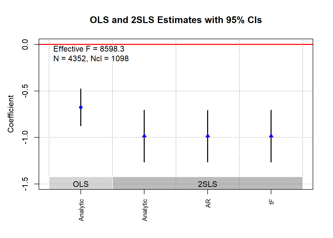
39.5.4 tF Procedure
Lee et al. (2022) introduce the tF procedure, an inference method specifically designed for just-identified IV models (single endogenous regressor and single instrument). It addresses the shortcomings of traditional 2SLS \(t\)-tests under weak instruments and offers a solution that is conceptually familiar to researchers trained in standard econometric practices.
Unlike the Anderson-Rubin test, which inverts hypothesis tests to form confidence sets, the tF procedure adjusts standard \(t\)-statistics and standard errors directly, making it a more intuitive extension of traditional hypothesis testing.
The tF procedure is widely applicable in settings where just-identified IV models arise, including:
Randomized controlled trials with imperfect compliance
(e.g., Local Average Treatment Effects in Imbens and Angrist (1994)).Fuzzy Regression Discontinuity Designs
(e.g., Lee and Lemieux (2010)).Fuzzy Regression Kink Designs
(e.g., (Card et al. 2015)).
A comparison of the AR approach and the tF procedure can be found in Andrews et al. (2019) (see also Table 39.6).
| Feature | Anderson-Rubin | tF Procedure |
|---|---|---|
| Robustness to Weak IV | Yes (valid under weak instruments) | Yes (valid under weak instruments) |
| Finite Confidence Intervals | No (interval becomes infinite for \(F \le 3.84\)) | Yes (finite intervals for all \(F\) values) |
| Interval Length | Often longer, especially when \(F\) is moderate (e.g., \(F = 16\)) | Typically shorter than AR intervals for \(F > 3.84\) |
| Ease of Interpretation | Requires inverting tests; less intuitive | Directly adjusts \(t\)-based standard errors; more intuitive |
| Computational Simplicity | Moderate (inversion of hypothesis tests) | Simple (multiplicative adjustment to standard errors) |
- With \(F > 3.84\), the AR test’s expected interval length is infinite, whereas the tF procedure guarantees finite intervals, making it superior in practical applications with weak instruments.
The tF procedure adjusts the conventional 2SLS \(t\)-ratio for the first-stage F-statistic strength. Instead of relying on a pre-testing threshold (e.g., \(F > 10\)), the tF approach provides a smooth adjustment to the standard errors.
Key Features:
- Adjusts the 2SLS \(t\)-ratio based on the observed first-stage F-statistic.
- Applies different adjustment factors for different significance levels (e.g., 95% and 99%).
- Remains valid even when the instrument is weak, offering finite confidence intervals even when the first-stage F-statistic is low.
Advantages of the tF Procedure
- Smooth Adjustment for First-Stage Strength
The tF procedure smoothly adjusts inference based on the observed first-stage F-statistic, avoiding the need for arbitrary pre-testing thresholds (e.g., \(F > 10\)).
-
It produces finite and usable confidence intervals even when the first-stage F-statistic is low:
\[ F > 3.84 \]
-
This threshold aligns with the critical value of 3.84 for a 95% Anderson-Rubin confidence interval, but with a crucial advantage:
- The AR interval becomes unbounded (i.e., infinite length) when \(F \le 3.84\).
- The tF procedure, in contrast, still provides a finite confidence interval, making it more practical in weak instrument cases.
- Clear and Interpretable Confidence Levels
-
The tF procedure offers transparent confidence intervals that:
Directly incorporate the impact of first-stage instrument strength on the critical values used for inference.
Mirror the distortion-free properties of robust methods like the Anderson-Rubin test, but remain closer in spirit to conventional \(t\)-based inference.
Researchers can interpret tF-based 95% and 99% confidence intervals using familiar econometric tools, without needing to invert hypothesis tests or construct confidence sets.
- Robustness to Common Error Structures
-
The tF procedure remains robust in the presence of:
- Heteroskedasticity
- Clustering
- Autocorrelation
-
No additional adjustments are necessary beyond the use of a robust variance estimator for both:
- The first-stage regression
- The second-stage IV regression
As long as the same robust variance estimator is applied consistently, the tF adjustment maintains valid inference without imposing additional computational complexity.
- Applicability to Published Research
-
One of the most powerful features of the tF procedure is its flexibility for re-evaluating published studies:
Researchers only need the reported first-stage F-statistic and standard errors from the 2SLS estimates.
No access to the original data is required to recalculate confidence intervals or test statistical significance using the tF adjustment.
-
This makes the tF procedure particularly valuable for meta-analyses, replications, and robustness checks of published IV studies, where:
- Raw data may be unavailable, or
- Replication costs are high.
Consider the linear IV model with additional covariates \(W\):
\[ Y = X \beta + W \gamma + u \]
\[ X = Z \pi + W \xi + \nu \]
Where:
\(Y\): Outcome variable.
\(X\): Endogenous regressor of interest.
\(Z\): Instrumental variable (single instrument case).
\(W\): Vector of exogenous controls, possibly including an intercept.
\(u\), \(\nu\): Error terms.
Key Statistics:
-
\(t\)-ratio for the IV estimator:
\[ \hat{t} = \frac{\hat{\beta} - \beta_0}{\sqrt{\hat{V}_N (\hat{\beta})}} \]
-
\(t\)-ratio for the first-stage coefficient:
\[ \hat{f} = \frac{\hat{\pi}}{\sqrt{\hat{V}_N (\hat{\pi})}} \]
-
First-stage F-statistic:
\[ \hat{F} = \hat{f}^2 \]
where
- \(\hat{\beta}\): Instrumental variable estimator.
- \(\hat{V}_N (\hat{\beta})\): Estimated variance of \(\hat{\beta}\), possibly robust to deal with non-iid errors.
- \(\hat{t}\): \(t\)-ratio under the null hypothesis.
- \(\hat{f}\): \(t\)-ratio under the null hypothesis of \(\pi=0\).
Under traditional asymptotics large samples, the \(t\)-ratio statistic follows:
\[ \hat{t}^2 \to^d t^2 \]
With critical values:
\(\pm 1.96\) for a 5% significance test.
\(\pm 2.58\) for a 1% significance test.
However, in IV settings (particularly with weak instruments):
The distribution of the \(t\)-statistic is distorted (i.e., \(t\)-distribution might not be normal), even in large samples.
The distortion arises because the strength of the instrument (\(F\)) and the degree of endogeneity (\(\rho\)) affect the \(t\)-distribution.
Stock and Yogo (2005) provide a formula to quantify this distortion (in the just-identified case) for Wald test statistics using 2SLS.:
\[ t^2 = f + t_{AR} + \rho f t_{AR} \]
Where:
\(\hat{f} \to^d f\)
\(\bar{f} = \dfrac{\pi}{\sqrt{\dfrac{1}{N} AV(\hat{\pi})}}\) and \(AV(\hat{\pi})\) is the asymptotic variance of \(\hat{\pi}\)
\(t_{AR}\) is asymptotically standard normal (\(AR = t^2_{AR}\))
\(\rho\) measures the correlation (degree of endogeneity) between \(Zu\) and \(Z\nu\) (when data are homoskedastic, \(\rho\) is the correlation between \(u\) and \(\nu\)).
Implications:
- For low \(\rho\) (\(\rho \in [0, 0.5]\)), rejection probabilities can be below nominal levels.
- For high \(\rho\) (\(\rho = 0.8\)), rejection rates can be inflated, e.g., 13% rejection at a nominal 5% significance level.
- Reliance on standard \(t\)-ratios leads to incorrect test sizes and invalid confidence intervals.
The tF procedure corrects for these distortions by adjusting the standard error of the 2SLS estimator based on the observed first-stage F-statistic.
Steps:
- Estimate \(\hat{\beta}\) and its conventional SE from 2SLS.
- Compute the first-stage \(\hat{F}\).
- Multiply the conventional SE by an adjustment factor, which depends on \(\hat{F}\) and the desired confidence level.
- Compute new \(t\)-ratios and construct confidence intervals using standard critical values (e.g., \(\pm 1.96\) for 95% CI).
Lee et al. (2022) refer to the adjusted standard errors as “0.05 tF SE” (for a 5% significance level) and “0.01 tF SE” (for 1%).
Lee et al. (2022) conducted a review of recent single-instrument studies in the American Economic Review.
Key Findings:
- For at least 25% of the examined specifications:
- tF-adjusted confidence intervals were 49% longer at the 5% level.
- tF-adjusted confidence intervals were 136% longer at the 1% level.
- Even among specifications with \(F > 10\) and \(t > 1.96\):
- Approximately 25% became statistically insignificant at the 5% level after applying the tF adjustment.
Takeaway:
- The tF procedure can substantially alter inference conclusions.
- Published studies can be re-evaluated with the tF method using only the reported first-stage F-statistics, without requiring access to the underlying microdata.
library(ivDiag)
g <- ivDiag::ivDiag(
    data = rueda,
    Y = "e_vote_buying",
    D = "lm_pob_mesa",
    Z = "lz_pob_mesa_f",
    controls = c("lpopulation", "lpotencial"),
    cl = "muni_code",
    cores = 4,
    bootstrap = FALSE
)
g$tF
#>         F        cF      Coef        SE         t    CI2.5%   CI97.5%   p-value
#> 8598.3264    1.9600   -0.9835    0.1424   -6.9071   -1.2626   -0.7044    0.0000
# example in fixest package
library(fixest)
library(tidyverse)
base = iris
names(base) = c("y", "x1", "x_endo_1", "x_inst_1", "fe")
set.seed(2)
base$x_inst_2 = 0.2 * base$y + 0.2 * base$x_endo_1 + rnorm(150, sd = 0.5)
base$x_endo_2 = 0.2 * base$y - 0.2 * base$x_inst_1 + rnorm(150, sd = 0.5)

est_iv = feols(y ~ x1 | x_endo_1 + x_endo_2 ~ x_inst_1 + x_inst_2, base)
est_iv
#> TSLS estimation - Dep. Var.: y
#>                   Endo.    : x_endo_1, x_endo_2
#>                   Instr.   : x_inst_1, x_inst_2
#> Second stage: Dep. Var.: y
#> Observations: 150
#> Standard-errors: IID
#>              Estimate Std. Error  t value   Pr(>|t|)
#> (Intercept)  1.831380   0.411435  4.45121 1.6844e-05 ***
#> fit_x_endo_1 0.444982   0.022086 20.14744  < 2.2e-16 ***
#> fit_x_endo_2 0.639916   0.307376  2.08186 3.9100e-02 *
#> x1           0.565095   0.084715  6.67051 4.9180e-10 ***
#> ---
#> Signif. codes:  0 '***' 0.001 '**' 0.01 '*' 0.05 '.' 0.1 ' ' 1
#> RMSE: 0.398842   Adj. R2: 0.725033
#> F-test (1st stage), x_endo_1: stat = 903.1628, p < 2.2e-16 , on 2 and 146 DoF.
#> F-test (1st stage), x_endo_2: stat =   3.2583, p = 0.041268, on 2 and 146 DoF.
#>                   Wu-Hausman: stat =   6.7918, p = 0.001518, on 2 and 144 DoF.

res_est_iv <- est_iv$coeftable |>
    rownames_to_column()


coef_of_interest <-
    res_est_iv[res_est_iv$rowname == "fit_x_endo_1", "Estimate"]
se_of_interest <-
    res_est_iv[res_est_iv$rowname == "fit_x_endo_1", "Std. Error"]
fstat_1st <- fitstat(est_iv, type = "ivf1")[[1]]$stat

# To get the correct SE based on 1st-stage F-stat (This result is similar without adjustment since F is large)
# the results are the new CIS and p.value
tF(coef = coef_of_interest, se = se_of_interest, Fstat = fstat_1st) |>
    causalverse::nice_tab(5)
#>          F   cF  Coef     SE       t CI2.5. CI97.5. p.value
#> 1 903.1628 1.96 0.445 0.0221 20.1474 0.4017  0.4883       0

# We can try to see a different 1st-stage F-stat and how it changes the results
tF(coef = coef_of_interest, se = se_of_interest, Fstat = 2) |>
    causalverse::nice_tab(5)
#>   F    cF  Coef     SE       t CI2.5. CI97.5. p.value
#> 1 2 18.66 0.445 0.0221 20.1474 0.0329  0.8571  0.0343
39.5.5 AK Approach
Angrist and Kolesár (2024) offer a reappraisal of just-identified IV models, focusing on the finite-sample properties of conventional inference in cases where a single instrument is used for a single endogenous variable. Their findings challenge some of the more pessimistic views about weak instruments and inference distortions in microeconometric applications.
Rather than propose a new estimator or test, Angrist and Kolesár provide a framework and rationale supporting the validity of traditional just-ID IV inference in many practical settings. Their insights clarify when conventional t-tests and confidence intervals can be trusted, and they offer practical guidance on first-stage pretesting, bias reduction, and endogeneity considerations.
AK apply their framework to three canonical studies:
- Angrist and Krueger (1991) - Education returns
- Angrist and Evans (1998) - Family size and female labor supply
- Angrist and Lavy (1999) - Class size effects
Findings:
Endogeneity (\(\rho\)) in these studies is moderate (typically \(|\rho| < 0.47\)).
Conventional t-tests and confidence intervals work reasonably well.
In many micro applications, theoretical bounds on causal effects and plausible OVB scenarios limit \(\rho\), supporting the validity of conventional inference.
Key Contributions of the AK Approach
Reassessing Bias and Coverage:
AK demonstrate that conventional IV estimates and t-tests in just-ID IV models often perform better than theory might suggest, provided the degree of endogeneity (\(\rho\)) is moderate, and the first-stage F-statistic is not extremely weak.-
First-Stage Sign Screening:
- They propose sign screening as a simple, costless strategy to halve the median bias of IV estimators.
- Screening on the sign of the estimated first-stage coefficient (i.e., using only samples where the first-stage estimate has the correct sign) improves the finite-sample performance of just-ID IV estimates without degrading confidence interval coverage.
-
Bias-Minimizing Screening Rule:
- AK show that setting the first-stage t-statistic threshold \(c = 0\), i.e., requiring only the correct sign of the first-stage estimate, minimizes median bias while preserving conventional coverage properties.
-
Practical Implication:
- They argue that conventional just-ID IV inference, including t-tests and confidence intervals, is likely valid in most microeconometric applications, especially where theory or institutional knowledge suggests the direction of the first-stage relationship.
39.5.5.1 Model Setup and Notation
AK adopt a reduced-form and first-stage specification for just-ID IV models:
\[ \begin{aligned} Y_i &= Z_i \delta + X_i' \psi_1 + u_i \\ D_i &= Z_i \pi + X_i' \psi_2 + v_i \end{aligned} \] where
- \(Y_i\): Outcome variable
- \(D_i\): Endogenous treatment variable
- \(Z_i\): Instrumental variable (single instrument)
- \(X_i\): Control variables
- \(u_i, v_i\): Error terms
Parameter of Interest:
\[ \beta = \frac{\delta}{\pi} \]
39.5.5.2 Endogeneity and Instrument Strength
AK characterize the two key parameters governing finite-sample inference:
Instrument Strength:
\[ E[F] = \frac{\pi^2}{\sigma^2_{\hat{\pi}}} + 1 \]
(Expected value of the first-stage F-statistic.)Endogeneity:
\[ \rho = \text{cor}(\hat{\delta} - \hat{\pi} \beta, \hat{\pi}) \]
Measures the degree of correlation between reduced-form and first-stage residuals (or between \(u\) and \(v\) under homoskedasticity).
Key Insight:
For \(\rho < 0.76\), the coverage of conventional 95% confidence intervals is distorted by less than 5%, regardless of the first-stage F-statistic.
39.5.5.3 First-Stage Sign Screening
AK argue that pre-screening based on the sign of the first-stage estimate (\(\hat{\pi}\)) offers bias reduction without compromising confidence interval coverage.
Screening Rule:
- Screen if \(\hat{\pi} > 0\)
(or \(\hat{\pi} < 0\) if the theoretical sign is negative).
Results:
- Halves median bias of the IV estimator.
- No degradation of confidence interval coverage.
This screening approach:
Avoids the pitfalls of pre-testing based on first-stage F-statistics (which can exacerbate bias and distort inference).
Provides a “free lunch”: bias reduction with no coverage cost.
39.5.5.4 Rejection Rates and Confidence Interval Coverage
- Rejection rates of conventional t-tests stay close to the nominal level (5%) if \(|\rho| < 0.76\), independent of instrument strength.
- For \(|\rho| < 0.565\), conventional t-tests exhibit no over-rejection, aligning with findings from Lee et al. (2022).
Comparison with AR and tF Procedures is summarised in Table 39.7.
| Approach | Bias Reduction | Coverage | CI Length (F > 3.84) |
|---|---|---|---|
| AK Sign Screening | Halves median bias | Near-nominal | Finite |
| AR Test | No bias (inversion method) | Exact | Infinite |
| tF Procedure | Bias adjusted | Near-nominal | Longer than AK (especially for moderate F) |
39.6 Testing Assumptions
We are interested in estimating the causal effect of an endogenous regressor \(X_2\) on an outcome variable \(Y\), using instrumental variables \(Z\) to address endogeneity.
The structural model of interest is:
\[ Y = \beta_1 X_1 + \beta_2 X_2 + \epsilon \]
- \(X_1\): Exogenous regressors
- \(X_2\): Endogenous regressor(s)
- \(Z\): Instrumental variables
If \(Z\) satisfies the relevance and exogeneity assumptions, we can identify \(\beta_2\) as:
\[ \beta_2 = \frac{Cov(Z, Y)}{Cov(Z, X_2)} \]
Alternatively, in terms of reduced form and first stage estimates:
- Reduced Form (effect of \(Z\) on \(Y\)):
\[ \rho = \frac{Cov(Y, Z)}{Var(Z)} \]
- First Stage (effect of \(Z\) on \(X_2\)):
\[ \pi = \frac{Cov(X_2, Z)}{Var(Z)} \]
- IV Estimate:
\[ \beta_2 = \frac{Cov(Y,Z)}{Cov(X_2, Z)} = \frac{\rho}{\pi} \]
To interpret \(\beta_2\) as the causal effect of \(X_2\) on \(Y\), the following assumptions must hold:
39.6.1 Relevance Assumption
In IV estimation, instrument relevance ensures that the instrument(s) \(Z\) can explain sufficient variation in the endogenous regressor(s) \(X_2\) to identify the structural equation:
\[ Y = \beta_1 X_1 + \beta_2 X_2 + \epsilon \]
The relevance condition requires that the instrument(s) \(Z\) be correlated with the endogenous variable(s) \(X_2\), conditional on other covariates \(X_1\). Formally:
\[ Cov(Z, X_2) \ne 0 \]
Or, in matrix notation for multiple instruments and regressors, the matrix of correlations (or more generally, the projection matrix) between \(Z\) and \(X_2\) must be of full column rank. This guarantees that \(Z\) has non-trivial explanatory power for \(X_2\).
An equivalent condition in terms of population moment conditions is that:
\[ E[Z' (X_2 - E[X_2 | Z])] \ne 0 \]
This condition ensures the identification of \(\beta_2\). Without it, the IV estimator would be undefined due to division by zero in its ratio form:
\[ \hat{\beta}_2^{IV} = \frac{Cov(Z, Y)}{Cov(Z, X_2)} \]
The first-stage regression operationalizes the relevance assumption:
\[ X_2 = Z \pi + X_1 \gamma + u \]
- \(\pi\): Vector of first-stage coefficients, measuring the effect of instruments on the endogenous regressor(s).
- \(u\): First-stage residual.
Identification of \(\beta_2\) requires that \(\pi \ne 0\). If \(\pi = 0\), the instrument has no explanatory power for \(X_2\), and the IV procedure collapses.
39.6.1.1 Weak Instruments
Even when \(Cov(Z, X_2) \ne 0\), weak instruments pose a serious problem in finite samples:
- Bias: The IV estimator becomes biased in the direction of the OLS estimator.
- Size distortion: Hypothesis tests can have inflated Type I error rates.
- Variance: Estimates become highly variable and unreliable.
Asymptotic vs. Finite Sample Problems
- IV estimators are consistent as \(n \to \infty\) if the relevance condition holds.
- With weak instruments, convergence can be so slow that finite-sample behavior is practically indistinguishable from inconsistency.
Boundaries between relevance and strength are thus critical in applied work.
39.6.1.2 First-Stage F-Statistic
In a single endogenous regressor case, the first-stage F-statistic is the standard test for instrument strength.
First-Stage Regression:
\[ X_2 = Z \pi + X_1 \gamma + u \]
We test:
\[ \begin{aligned} H_0&: \pi = 0 \quad \text{(Instruments have no explanatory power)} \\ H_1&: \pi \ne 0 \quad \text{(Instruments explain variation in $X_2$)} \end{aligned} \]
F-Statistic Formula:
\[ F = \frac{(SSR_r - SSR_{ur}) / q}{SSR_{ur} / (n - k - 1)} \]
- \(SSR_r\): Sum of squared residuals from the restricted model (no instruments).
- \(SSR_{ur}\): Sum of squared residuals from the unrestricted model (with instruments).
- \(q\): Number of excluded instruments (restrictions tested).
- \(n\): Number of observations.
- \(k\): Number of control variables.
Interpretation has accumulated layers of guidance over the years, and it is worth tracing them rather than treating the F-statistic as a single-number verdict. The original rule of thumb is Staiger and Stock (1997): if \(F < 10\), declare the instruments weak and treat the 2SLS estimates with suspicion. That heuristic has held up culturally but has worn poorly statistically. Lee et al. (2022) show that the conventional threshold is too permissive, confidence intervals built around 2SLS estimates with \(F\) in the 10-20 range can undercover badly, and they advocate model-specific diagnostics in place of the universal cutoff. When weakness is a serious concern, the recommended remedy is to switch from the 2SLS \(t\)-statistic to weak-instrument-robust inference; the Conditional Likelihood Ratio test of Moreira (2003; Andrews et al. 2008) is the standard tool for this and should be the default whenever the first-stage strength is in doubt.
Use linearHypothesis() in R to test instrument relevance.
39.6.1.3 Cragg-Donald Test
The Cragg-Donald statistic is essentially the same as the Wald statistic of the joint significance of the instruments in the first stage (Cragg and Donald 1993), and it’s used specifically when you have multiple endogenous regressors. It’s calculated as:
\[ CD = n \times (R_{ur}^2 - R_r^2) \]
where:
\(R_{ur}^2\) and \(R_r^2\) are the R-squared values from the unrestricted and restricted models respectively.
\(n\) is the number of observations.
For one endogenous variable, the Cragg-Donald test results should align closely with those from Stock and Yogo. The Anderson canonical correlation test, a likelihood ratio test, also works under similar conditions, contrasting with Cragg-Donald’s Wald statistic approach. Both are valid with one endogenous variable and at least one instrument.
library(cragg)
library(AER) # for dataaset
data("WeakInstrument")

cragg_donald(
    # control variables
    X = ~ 1,
    # endogeneous variables
    D = ~ x,
    # instrument variables
    Z = ~ z,
    data = WeakInstrument
)
#> Cragg-Donald test for weak instruments:
#>
#>      Data:                        WeakInstrument
#>      Controls:                    ~1
#>      Treatments:                  ~x
#>      Instruments:                 ~z
#>
#>      Cragg-Donald Statistic:        4.566136
#>      Df:                                 198
Large CD statistic implies that the instruments are strong, but not in our case here. But to judge it against some critical value, we have to look at Stock-Yogo
39.6.1.4 Stock-Yogo
The Stock-Yogo test does not directly compute a statistic like the F-test or Cragg-Donald, but rather uses pre-computed critical values to assess the strength of instruments. It often uses the eigenvalues derived from the concentration matrix:
\[ S = \frac{1}{n} (Z' X) (X'Z) \]
where \(Z\) is the matrix of instruments and \(X\) is the matrix of endogenous regressors.
Stock and Yogo provide critical values for different scenarios (bias, size distortion) for a given number of instruments and endogenous regressors, based on the smallest eigenvalue of \(S\). The test compares these eigenvalues against critical values that correspond to thresholds of permissible bias or size distortion in a 2SLS estimator.
- Critical Values and Test Conditions: The critical values derived by Stock and Yogo depend on the level of acceptable bias, the number of endogenous regressors, and the number of instruments. For example, with a 5% maximum acceptable bias, one endogenous variable, and three instruments, the critical value for a sufficient first stage F-statistic is 13.91. Note that this framework requires at least two overidentifying degree of freedom. Stock and Yogo (2002) set the critical values such that the bias is less than 10% (default)
\(H_0:\) Instruments are weak
\(H_1:\) Instruments are not weak
library(cragg)
library(AER) # for dataaset
data("WeakInstrument")

stock_yogo_test(
    # control variables
    X =  ~ Sepal.Length,
    # endogeneous variables
    D =  ~ Sepal.Width,
    # instrument variables
    Z =  ~ Petal.Length + Petal.Width + Species,
    size_bias = "bias",
    data = iris
)
#> Results of Stock and Yogo test for weak instruments:
#>
#>      Null Hypothesis:             Instruments are weak
#>      Alternative Hypothesis:      Instruments are not weak
#>
#>      Data:                        iris
#>      Controls:                    ~Sepal.Length
#>      Treatments:                  ~Sepal.Width
#>      Instruments:                 ~Petal.Length + Petal.Width + Species
#>
#>      Alpha:                             0.05
#>      Acceptable level of bias:    5% relative to OLS.
#>      Critical Value:                   16.85
#>
#>      Cragg-Donald Statistic:        61.30973
#>      Df:                                 144
39.6.1.5 Anderson-Rubin Test
The Anderson-Rubin (AR) test addresses the issues of weak instruments by providing a test for the structural parameter (\(\beta\)) that is robust to weak instruments (Anderson and Rubin 1949). It does not rely on the strength of the instruments to control size, making it a valuable tool for inference when instrument relevance is questionable.
Consider the following linear IV model:
\[ Y = X \beta + u \]
- \(Y\): Dependent variable (\(n \times 1\))
- \(X\): Endogenous regressor (\(n \times k\))
-
\(Z\): Instrument matrix (\(n \times m\)), assumed to satisfy:
- Instrument Exogeneity: \(\mathbb{E}[Z'u] = 0\)
- Instrument Relevance: \(\mathrm{rank}(\mathbb{E}[Z'X]) = k\)
The relevance assumption ensures that \(Z\) contains valid information for predicting \(X\).
Relevance is typically assessed in the first-stage regression:
\[ X = Z \Pi + V \]
If \(Z\) is weakly correlated with \(X\), \(\Pi\) is close to zero, violating the relevance assumption.
The AR test is a Wald-type test for the null hypothesis:
\[ H_0: \beta = \beta_0 \]
It is constructed by examining whether the residuals from imposing \(\beta_0\) are orthogonal to the instruments \(Z\). Specifically:
- Compute the reduced-form residuals under \(H_0\):
\[ r(\beta_0) = Y - X \beta_0 \]
- The AR test statistic is:
\[ AR(\beta_0) = \frac{r(\beta_0)' P_Z r(\beta_0)}{\hat{\sigma}^2} \]
- \(P_Z = Z (Z'Z)^{-1} Z'\) is the projection matrix onto the column space of \(Z\).
- \(\hat{\sigma}^2 = \frac{r(\beta_0)' M_Z r(\beta_0)}{n - m}\) is the residual variance estimator, with \(M_Z = I - P_Z\).
Under \(H_0\), and assuming homoskedasticity, the AR statistic follows an F-distribution:
\[ AR(\beta_0) \sim F(m, n - m) \]
Alternatively, for large \(n\), the AR statistic can be approximated by a chi-squared distribution:
\[ AR(\beta_0) \sim \chi^2_m \]
Interpretation
- If \(AR(\beta_0)\) exceeds the critical value from the \(F\) (or \(\chi^2\)) distribution, we reject \(H_0\).
- The test assesses whether \(r(\beta_0)\) is orthogonal to \(Z\). If not, \(H_0\) is inconsistent with the moment conditions.
The key advantage of the AR test is that its size is correct even when instruments are weak. The AR statistic does not depend on the strength of the instruments (i.e., the magnitude of \(\Pi\)), making it valid under weak identification.
This contrasts with standard 2SLS-based Wald tests, whose distribution depends on the first-stage relevance and can be severely distorted if \(Z\) is weakly correlated with \(X\).
- The relevance assumption is necessary for point identification and consistent estimation in IV.
- If instruments are weak, point estimates of \(\beta\) from 2SLS can be biased.
- The AR test allows for valid hypothesis testing, even if instrument relevance is weak.
However, if instruments are completely irrelevant (i.e., \(Z'X = 0\)), the IV model is unidentified, and the AR test lacks power (i.e., it does not reject \(H_0\) for any \(\beta_0\)).
The AR test can be inverted to form confidence sets for \(\beta\):
- Compute \(AR(\beta)\) for a grid of \(\beta\) values.
- Include all \(\beta\) values for which \(AR(\beta)\) does not reject \(H_0\) at the chosen significance level.
These confidence sets are robust to weak instruments and can be disconnected or unbounded if identification is weak.
set.seed(123)

# Simulate data
n <- 500
Z <- cbind(1, rnorm(n)) # Instrument (include constant)
X <- 0.1 * Z[,2] + rnorm(n) # Weak first-stage relationship
beta_true <- 1
u <- rnorm(n)
Y <- X * beta_true + u


library(ivmodel)
ivmodel(Y = Y, D = X, Z = Z)
#>
#> Call:
#> ivmodel(Y = Y, D = X, Z = Z)
#> sample size: 500
#> _ _ _ _ _ _ _ _ _ _ _ _ _ _ _ _ _ _ _ _ _ _ _ _ _ _ _ _ _ _
#>
#> First Stage Regression Result:
#>
#> F=0.684842, df1=2, df2=497, p-value is 0.50464
#> R-squared=0.002748329,   Adjusted R-squared=-0.001264756
#> Residual standard error: 1.01117 on 499 degrees of freedom
#> _ _ _ _ _ _ _ _ _ _ _ _ _ _ _ _ _ _ _ _ _ _ _ _ _ _ _ _ _ _
#>
#> Sargan Test Result:
#>
#> Sargan Test Statistics=0.007046677, df=1, p-value is 0.9331
#> _ _ _ _ _ _ _ _ _ _ _ _ _ _ _ _ _ _ _ _ _ _ _ _ _ _ _ _ _ _
#>
#> Coefficients of k-Class Estimators:
#>
#>              k Estimate Std. Error t value Pr(>|t|)
#> OLS    0.00000  1.05559    0.04396  24.015   <2e-16 ***
#> Fuller 0.99800  1.81913    0.80900   2.249   0.0250 *
#> TSLS   1.00000  2.37533    1.40555   1.690   0.0917 .
#> LIML   1.00001  2.38211    1.41382   1.685   0.0926 .
#> ---
#> Signif. codes:  0 '***' 0.001 '**' 0.01 '*' 0.05 '.' 0.1 ' ' 1
#> _ _ _ _ _ _ _ _ _ _ _ _ _ _ _ _ _ _ _ _ _ _ _ _ _ _ _ _ _ _
#>
#> Alternative tests for the treatment effect under H_0: beta=0.
#>
#> Anderson-Rubin test (under F distribution):
#> F=1.874305, df1=2, df2=497, p-value is 0.15454
#> 95 percent confidence interval:
#>  Whole Real Line
#>
#> Conditional Likelihood Ratio test (under Normal approximation):
#> Test Stat=3.741629, p-value is 0.14881
#> 95 percent confidence interval:
#>  Whole Real Line
39.6.1.6 Stock-Wright Test
While the Anderson-Rubin test offers one solution by constructing test statistics that are valid regardless of instrument strength, another complementary approach is the Stock-Wright test, sometimes referred to as the S-test or Score test. This test belongs to a broader class of conditional likelihood ratio tests proposed by Moreira (2003) and Stock and Wright (2000), and it plays an important role in constructing weak-instrument robust confidence regions.
The Stock-Wright test exploits the conditional score function of the IV model to test hypotheses about structural parameters, offering robustness under weak identification.
Consider the linear IV model:
\[ Y = X \beta + u \]
- \(Y\): Outcome variable (\(n \times 1\))
- \(X\): Endogenous regressor (\(n \times k\))
- \(Z\): Instrument matrix (\(n \times m\)), where \(m \ge k\)
The exogeneity and relevance assumptions for \(Z\) are:
- \(\mathbb{E}[Z'u] = 0\) (Exogeneity)
- \(\mathrm{rank}(\mathbb{E}[Z'X]) = k\) (Relevance)
Weak instruments imply that the matrix \(\mathbb{E}[Z'X]\) is close to rank-deficient or nearly zero, which can invalidate standard inference.
The goal is to test the null hypothesis:
\[ H_0: \beta = \beta_0 \]
The Stock-Wright test provides a robust way to perform this hypothesis test by constructing a score statistic that is robust to weak instruments.
The score test (or Lagrange Multiplier test) evaluates whether the score (the gradient of the log-likelihood function with respect to \(\beta\)) is close to zero under the null hypothesis.
In the IV context, the conditional score is evaluated from the reduced-form equations. The SW test uses the fact that under \(H_0\), the moment condition:
\[ \mathbb{E}[Z'(Y - X \beta_0)] = 0 \]
should hold. Deviations from this condition can be tested using a score statistic.
The reduced-form equations are:
\[ \begin{aligned} Y &= Z \pi_Y + \epsilon_Y \\ X &= Z \pi_X + \epsilon_X \end{aligned} \]
Under this system:
\(\epsilon_Y\) and \(\epsilon_X\) are jointly normally distributed with covariance matrix \(\Sigma\).
The structural model implies a restriction on \(\pi_Y\): \(\pi_Y = \pi_X \beta\).
The Stock-Wright test statistic is given by:
\[ S(\beta_0) = (Z'(Y - X \beta_0))' \left[ \hat{\Omega}^{-1} \right] (Z'(Y - X \beta_0)) \]
Where:
\(\hat{\Omega}\) is an estimator of the covariance matrix of the moment condition \(Z'u\), often estimated by \(Z'Z\) times an estimator of \(\mathrm{Var}(u)\).
In homoskedastic settings, \(\hat{\Omega} = \hat{\sigma}^2 Z'Z\), with \(\hat{\sigma}^2\) estimated from the residuals under \(H_0\):
\[ \hat{\sigma}^2 = \frac{(Y - X \beta_0)' (Y - X \beta_0)}{n} \]
Under the null hypothesis \(H_0\), the test statistic \(S(\beta_0)\) follows a chi-squared distribution with \(m\) degrees of freedom:
\[ S(\beta_0) \sim \chi^2_m \]
The Stock-Wright test is closely related to the Anderson-Rubin test. However:
- The AR test focuses on the orthogonality of the reduced-form residuals with \(Z\).
- The SW test focuses on the conditional score, derived from the likelihood framework.
- Both are robust to weak instruments, but they have different power properties depending on the data-generating process.
Geometric Intuition
- The SW test can be seen as testing whether the orthogonality condition between \(Z\) and \(u\) holds, using a score function.
- It effectively checks whether the directional derivative of the likelihood (evaluated at \(\beta_0\)) is zero, offering a generalized method of moments interpretation.
The Stock-Wright S-test can be inverted to form confidence regions:
- For a grid of \(\beta\) values, compute \(S(\beta)\).
- The confidence region consists of all \(\beta\) values where \(S(\beta)\) does not reject \(H_0\) at the chosen significance level.
These regions are robust to weak instruments, and can be disconnected or unbounded if the instruments are too weak to deliver informative inference.
set.seed(42)

# Simulate data
n <- 500
Z <- cbind(1, rnorm(n)) # Instrument (include constant)
X <- 0.1 * Z[,2] + rnorm(n) # Weak first-stage relationship
beta_true <- 1
u <- rnorm(n)
Y <- X * beta_true + u

# Null hypothesis to test
beta_0 <- 0

# Residuals under H0
r_beta0 <- Y - X * beta_0

# Estimate variance of residuals under H0
sigma2_hat <- mean(r_beta0^2)

# Compute Omega matrix
Omega_hat <- sigma2_hat * t(Z) %*% Z

# Compute the Stock-Wright S-statistic
S_stat <- t(t(Z) %*% r_beta0) %*% solve(Omega_hat) %*% (t(Z) %*% r_beta0)

# p-value from chi-squared distribution
df <- ncol(Z) # degrees of freedom
p_val <- 1 - pchisq(S_stat, df = df)

# Output
cat("Stock-Wright S-Statistic:", round(S_stat, 4), "\n")
#> Stock-Wright S-Statistic: 5.0957
cat("p-value:", round(p_val, 4), "\n")
#> p-value: 0.0783
39.6.1.7 Kleibergen-Paap rk Statistic
Traditional diagnostics for instrument relevance, such as:
The first-stage \(F\)-statistic (for single endogenous variables with homoskedastic errors)
The Cragg-Donald statistic (for multiple endogenous regressors under homoskedasticity)
are not valid when errors exhibit heteroskedasticity or non-i.i.d. behavior.
The Kleibergen-Paap (KP) rk statistic addresses these limitations by providing a robust test for underidentification and weak identification in IV models, even in the presence of heteroskedasticity.
Consider the linear IV model:
\[ Y = X \beta + u \]
- \(Y\): Dependent variable (\(n \times 1\))
- \(X\): Matrix of endogenous regressors (\(n \times k\))
- \(Z\): Instrument matrix (\(n \times m\)), with \(m \ge k\)
- \(u\): Structural error term
The moment conditions under exogeneity are:
\[ \mathbb{E}[Z'u] = 0 \]
The relevance assumption requires:
\[ \mathrm{rank}(\mathbb{E}[Z'X]) = k \]
If this condition fails, the model is underidentified, and consistent estimation of \(\beta\) is impossible.
The Kleibergen-Paap rk statistic performs two key functions:
- Test for underidentification (whether the instruments identify the equation)
- Weak identification diagnostics, analogous to the Cragg-Donald statistic, but robust to heteroskedasticity.
Why “rk”?
- “rk” stands for rank: the statistic tests whether the matrix of reduced-form coefficients has full rank, necessary for identification.
The KP rk statistic builds on the generalized method of moments framework and the canonical correlations between \(X\) and \(Z\).
The reduced-form for \(X\) is:
\[ X = Z \Pi + V \]
- \(\Pi\): Matrix of reduced-form coefficients (\(m \times k\))
- \(V\): First-stage residuals (\(n \times k\))
Under the null hypothesis of underidentification, the matrix \(\Pi\) is rank deficient, meaning \(\Pi\) does not have full rank \(k\).
The Kleibergen-Paap rk statistic tests the null hypothesis:
\[ H_0: \mathrm{rank}(\mathbb{E}[Z'X]) < k \]
Against the alternative:
\[ H_A: \mathrm{rank}(\mathbb{E}[Z'X]) = k \]
The Kleibergen-Paap rk statistic is a Lagrange Multiplier test statistic derived from the first-stage canonical correlations between \(X\) and \(Z\), adjusted for heteroskedasticity.
Computation Outline
- Compute first-stage residuals for each endogenous regressor.
- Estimate the covariance matrix of the residuals, allowing for heteroskedasticity.
- Calculate the rank test statistic, which has an asymptotic chi-squared distribution with \(k(m - k)\) degrees of freedom.
Under \(H_0\), the KP rk statistic follows:
\[ KP_{rk} \sim \chi^2_{k(m - k)} \]
Intuition Behind the KP rk Statistic
- The statistic examines whether the moment conditions based on \(Z\) provide enough information to identify \(\beta\).
- If \(Z\) fails to explain sufficient variation in \(X\), the instruments are not relevant, and the model is underidentified.
- The KP rk test is a necessary condition for relevance, though not a sufficient measure of instrument strength.
Practical Usage
- A rejection of \(H_0\) suggests that the instruments are relevant enough for identification.
- A failure to reject \(H_0\) implies underidentification, and the IV estimates are not valid.
While the KP rk statistic tests for underidentification, it does not directly assess weak instruments. However, it is often reported alongside Kleibergen-Paap LM and Wald statistics, which address weak instrument diagnostics in heteroskedastic settings.
Comparison: Kleibergen-Paap rk vs Cragg-Donald Statistic, summarised in Table 39.8.
| Feature | Kleibergen-Paap rk Statistic | Cragg-Donald Statistic |
|---|---|---|
| Robust to Heteroskedasticity | Yes | No |
| Valid Under Non-i.i.d. Errors | Yes | No |
| Underidentification Test | Yes | No (tests weak instruments) |
| Degrees of Freedom | \(k(m - k)\) | Varies (depends on \(k\) and \(m\)) |
| Applicability | Always preferred in practice | Homoskedastic errors only |
# Load necessary packages
library(sandwich)  # For robust covariance estimators
library(lmtest)    # For testing
library(AER)       # For IV estimation (optional)

# Simulate data
set.seed(123)
n <- 500
Z1 <- rnorm(n)
Z2 <- rnorm(n)
Z <- cbind(1, Z1, Z2) # Instruments (include intercept)

# Weak instrument case
X1 <- 0.1 * Z1 + 0.1 * Z2 + rnorm(n)
X <- cbind(X1)
beta_true <- 1
u <- rnorm(n)
Y <- X %*% beta_true + u

# First-stage regression: X ~ Z
first_stage <- lm(X1 ~ Z1 + Z2)
V <- residuals(first_stage) # First-stage residuals

# Calculate robust covariance matrix of residuals
# Note: sandwich package already computes heteroskedasticity-consistent covariances

# Kleibergen-Paap rk test via sandwich estimators (conceptual)
# In practice, Kleibergen-Paap rk statistics are provided by ivreg2 (Stata) or via custom functions

# For illustration, using ivreg and summary statistics
iv_model <- ivreg(Y ~ X1 | Z1 + Z2)

# Kleibergen-Paap rk statistic (reported by summary under diagnostics)
summary(iv_model, diagnostics = TRUE)
#>
#> Call:
#> ivreg(formula = Y ~ X1 | Z1 + Z2)
#>
#> Residuals:
#>        Min         1Q     Median         3Q        Max
#> -3.2259666 -0.6433047  0.0004169  0.8384112  3.4831350
#>
#> Coefficients:
#>             Estimate Std. Error t value Pr(>|t|)
#> (Intercept)  0.05389    0.04810   1.120    0.263
#> X1           1.16437    0.22129   5.262 2.12e-07 ***
#>
#> Diagnostic tests:
#>                  df1 df2 statistic  p-value
#> Weak instruments   2 497    11.793 9.91e-06 ***
#> Wu-Hausman         1 497     2.356  0.12541
#> Sargan             1  NA     6.934  0.00846 **
#> ---
#> Signif. codes:  0 '***' 0.001 '**' 0.01 '*' 0.05 '.' 0.1 ' ' 1
#>
#> Residual standard error: 1.066 on 498 degrees of freedom
#> Multiple R-Squared: 0.3593,  Adjusted R-squared: 0.358
#> Wald test: 27.69 on 1 and 498 DF,  p-value: 2.123e-07

# Interpretation:
# Weak instruments are flagged if the KP rk statistic does not reject underidentification.
Interpretation
The Kleibergen-Paap rk statistic is reported alongside LM and Wald weak identification tests.
The p-value of the rk statistic tells us whether the equation is identified.
If the test rejects, we proceed to evaluate weak instrument strength using Wald or LM statistics.
39.6.1.8 Comparison of Weak Instrument Tests
Table 39.9 compares the main weak-instrument diagnostics on description, use case, and assumptions.
| Test | Description | Use Case | Assumptions |
|---|---|---|---|
| First-Stage F-Statistic | Joint significance of instruments on \(X_2\) | Simple IV models (1 endogenous regressor, 1+ instruments) | i.i.d. errors |
| Cragg-Donald Wald | Wald test for multiple instruments and endogenous variables | Multi-equation IV models | i.i.d. errors |
| Stock-Yogo | Critical values for bias/size distortion | Assess bias and size distortions in 2SLS estimator | i.i.d. errors |
| Anderson-Rubin | Joint significance test in structural equation | Robust to weak instruments; tests hypotheses on \(\beta_2\) | None (valid under weak IV) |
| Kleinbergen-Paap rk | Generalized Cragg-Donald for heteroskedastic/clustered errors | Robust inference when classical assumptions fail; heteroskedastic-consistent inference | Allows heteroskedasticity |
All the mentioned tests (Stock Yogo, Cragg-Donald, Anderson canonical correlation test) assume errors are independently and identically distributed. If this assumption is violated, the Kleinbergen-Paap test is robust against violations of the iid assumption and can be applied even with a single endogenous variable and instrument, provided the model is properly identified (Baum and Lewbel 2019).
39.6.2 Independence (Unconfoundedness)
- \(Z\) is independent of any factors affecting \(Y\), apart from through \(X_2\).
- Formally: \(Z \perp \epsilon\).
This is stronger than exclusion restriction and typically requires randomized assignment of \(Z\) or strong theoretical justification.
39.6.3 Monotonicity Assumption
- Relevant for identifying Local Average Treatment Effects (Imbens and Angrist 1994)
- Assumes there are no defiers: the instrument \(Z\) does not cause the treatment \(X_2\) to increase for some units while decreasing it for others.
\[ X_2(Z = 1) \ge X_2(Z = 0) \quad \text{for all individuals} \]
- Ensures we are identifying a [Local Average Treatment Effect] (LATE) for the group of compliers, individuals whose treatment status responds to the instrument.
This assumption is particularly important in empirical applications involving binary instruments and heterogeneous treatment effects.
In business settings, instruments often arise from policy changes, eligibility cutoffs, or randomized marketing campaigns. For instance:
- A firm rolls out a new loyalty program (\(Z = 1\)) in selected regions to encourage purchases (\(X_2\)). The monotonicity assumption implies that no customer reduces their purchases because of the program; it only increases them or leaves them unchanged.
This assumption rules out defiers (individuals who respond to the instrument in the opposite direction), which would otherwise bias the IV estimate by introducing effects not attributable to compliers. Violations of monotonicity make the IV estimate difficult to interpret, as it may average over both compliers and defiers, yielding a non-causal or ambiguous LATE.
While monotonicity is an assumption about unobserved counterfactuals and thus not directly testable, several empirical strategies can provide suggestive evidence:
- First-Stage Regression
Estimate the impact of the instrument on the treatment. A strong, consistent sign across subgroups supports monotonicity.
set.seed(123)

# Sample size
n <- 1000

# Generate instrument (Z), treatment (D), and outcome (Y)
Z <- rbinom(n, 1, 0.5)  # Binary instrument (e.g., policy change)
U <- rnorm(n)           # Unobserved confounder
D <- 0.8 * Z + 0.3 * U + rnorm(n)  # Treatment variable
Y <- 2 * D + 0.5 * U + rnorm(n)    # Outcome variable

# Create a data frame
df <- data.frame(Z, D, Y)

# First-stage regression
first_stage <- lm(D ~ Z, data = df)
summary(first_stage)
#>
#> Call:
#> lm(formula = D ~ Z, data = df)
#>
#> Residuals:
#>     Min      1Q  Median      3Q     Max
#> -3.2277 -0.7054  0.0105  0.7047  3.3846
#>
#> Coefficients:
#>             Estimate Std. Error t value Pr(>|t|)
#> (Intercept)  0.02910    0.04651   0.626    0.532
#> Z            0.74286    0.06623  11.216   <2e-16 ***
#> ---
#> Signif. codes:  0 '***' 0.001 '**' 0.01 '*' 0.05 '.' 0.1 ' ' 1
#>
#> Residual standard error: 1.047 on 998 degrees of freedom
#> Multiple R-squared:  0.1119, Adjusted R-squared:  0.111
#> F-statistic: 125.8 on 1 and 998 DF,  p-value: < 2.2e-16

# Check F-statistic
fs_f_stat <- summary(first_stage)$fstatistic[1]
fs_f_stat
#>    value
#> 125.7911
A positive and significant coefficient on \(Z\) supports a monotonic relationship.
If the coefficient is near zero or flips sign in subgroups, this may signal violations.
- Density Plot of First-Stage Residuals
Figure 39.1 shows the density of first-stage residuals. A unimodal shape supports the monotonicity assumption, whereas a bimodal or heavily skewed pattern would suggest a mixture of compliers and defiers.
# Extract residuals
residuals_first_stage <- residuals(first_stage)

# Plot density
library(ggplot2)
ggplot(data.frame(residuals = residuals_first_stage),
       aes(x = residuals)) +
    geom_density(fill = "blue", alpha = 0.5) +
    ggtitle("Density of First-Stage Residuals") +
    xlab("Residuals from First-Stage Regression") +
    ylab("Density") +
    causalverse::ama_theme()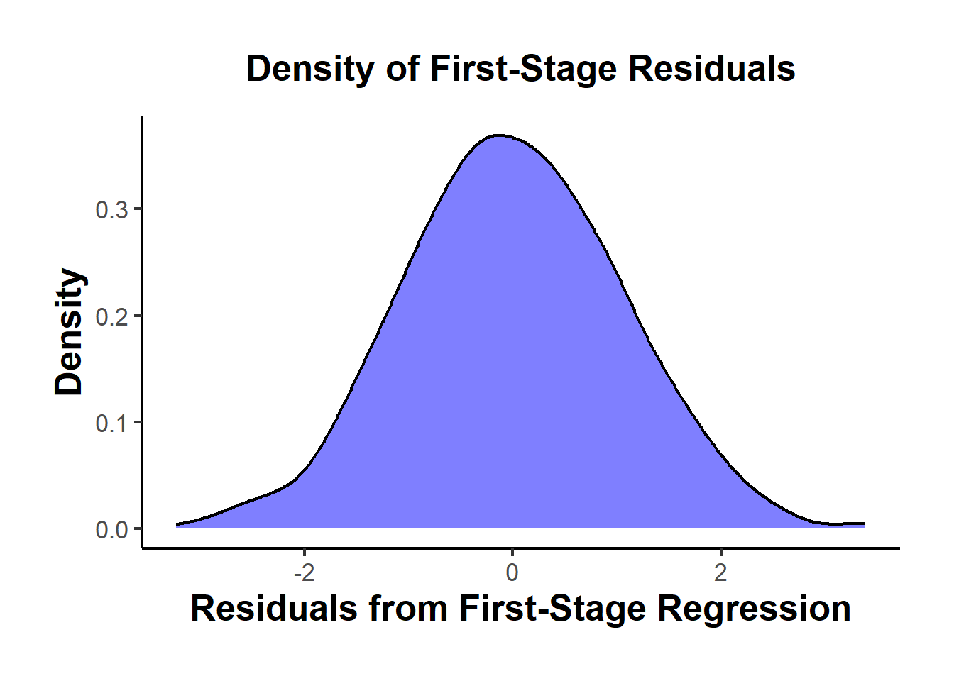
Figure 39.1: Density of first-stage residuals; a unimodal shape supports monotonicity of the instrument, whereas a bimodal or heavily skewed pattern hints at compliers mixed with defiers.
A unimodal residual distribution supports monotonicity.
A bimodal or heavily skewed pattern could suggest a mixture of compliers and defiers.
- Subgroup Analysis
Split the sample into subgroups (e.g., by market segment or region) and compare the first-stage coefficients.
# Create two random subgroups
df$subgroup <- ifelse(runif(n) > 0.5, "Group A", "Group B")

# First-stage regression in subgroups
first_stage_A <- lm(D ~ Z, data = df[df$subgroup == "Group A", ])
first_stage_B <- lm(D ~ Z, data = df[df$subgroup == "Group B", ])

# Compare coefficients
coef_A <- coef(first_stage_A)["Z"]
coef_B <- coef(first_stage_B)["Z"]

cat("First-stage coefficient for Group A:", coef_A, "\n")
#> First-stage coefficient for Group A: 0.6645617
cat("First-stage coefficient for Group B:", coef_B, "\n")
#> First-stage coefficient for Group B: 0.8256711
If both groups show a coefficient with the same sign, this supports monotonicity.
Opposing signs raise concerns that some individuals may respond against the instrument.
39.6.4 Homogeneous Treatment Effects (Optional)
- Assumes that the causal effect of \(X_2\) on \(Y\) is constant across individuals.
- Without this, IV estimates a local rather than global average treatment effect (LATE vs ATE).
39.6.5 Linearity and Additivity
- The functional form is linear in parameters:
\[ Y = X \beta + \epsilon \]
- No interactions or non-linearities unless explicitly modeled.
- Additivity of the error term \(\epsilon\) implies no heteroskedasticity in classic IV models (though robust standard errors can relax this).
39.6.6 Instrument Exogeneity (Exclusion Restriction)
- \(E[Z \epsilon] = 0\): Instruments must not be correlated with the error term.
- \(Z\) influences \(Y\) only through \(X_2\).
- No omitted variable bias from unobserved confounders correlated with \(Z\).
Key Interpretation:
- \(Z\) has no direct effect on \(Y\).
- Any pathway from \(Z\) to \(Y\) must operate exclusively through \(X_2\).
39.6.7 Exogeneity Assumption
The local average treatment effect (LATE) is defined as:
\[ \text{LATE} = \frac{\text{reduced form}}{\text{first stage}} = \frac{\rho}{\phi} \]
This implies that the reduced form (\(\rho\)) is the product of the first stage (\(\phi\)) and LATE:
\[ \rho = \phi \times \text{LATE} \]
Thus, if the first stage (\(\phi\)) is 0, the reduced form (\(\rho\)) should also be 0.
The skeleton below describes a Shiny app that simulates the IV model and displays first-stage, reduced-form, calculated-LATE, and IV-LATE coefficients with confidence intervals as the user varies the true effect, the first-stage strength, and the direct effect of the instrument on the outcome.
# Load necessary libraries
library(shiny)
library(AER)  # for ivreg
library(ggplot2)  # for visualization
library(dplyr)  # for data manipulation

# Function to simulate the dataset
simulate_iv_data <- function(n, beta, phi, direct_effect) {
  Z <- rnorm(n)
  epsilon_x <- rnorm(n)
  epsilon_y <- rnorm(n)
  X <- phi * Z + epsilon_x
  Y <- beta * X + direct_effect * Z + epsilon_y
  data <- data.frame(Y = Y, X = X, Z = Z)
  return(data)
}

# Function to run the simulations and calculate the effects
run_simulation <- function(n, beta, phi, direct_effect) {
  # Simulate the data
  simulated_data <- simulate_iv_data(n, beta, phi, direct_effect)

  # Estimate first-stage effect (phi)
  first_stage <- lm(X ~ Z, data = simulated_data)
  phi <- coef(first_stage)["Z"]
  phi_ci <- confint(first_stage)["Z", ]

  # Estimate reduced-form effect (rho)
  reduced_form <- lm(Y ~ Z, data = simulated_data)
  rho <- coef(reduced_form)["Z"]
  rho_ci <- confint(reduced_form)["Z", ]

  # Estimate LATE using IV regression
  iv_model <- ivreg(Y ~ X | Z, data = simulated_data)
  iv_late <- coef(iv_model)["X"]
  iv_late_ci <- confint(iv_model)["X", ]

  # Calculate LATE as the ratio of reduced-form and first-stage coefficients
  calculated_late <- rho / phi
  calculated_late_se <- sqrt(
    (rho_ci[2] - rho)^2 / phi^2 + (rho * (phi_ci[2] - phi) / phi^2)^2
  )
  calculated_late_ci <- c(calculated_late - 1.96 * calculated_late_se,
                          calculated_late + 1.96 * calculated_late_se)

  # Return a list of results
  list(phi = phi,
       phi_ci = phi_ci,
       rho = rho,
       rho_ci = rho_ci,
       direct_effect = direct_effect,
       direct_effect_ci = c(direct_effect, direct_effect),  # Placeholder for direct effect CI
       iv_late = iv_late,
       iv_late_ci = iv_late_ci,
       calculated_late = calculated_late,
       calculated_late_ci = calculated_late_ci,
       true_effect = beta,
       true_effect_ci = c(beta, beta))  # Placeholder for true effect CI
}

# Define UI for the sliders
ui <- fluidPage(
  titlePanel("IV Model Simulation"),
  sidebarLayout(
    sidebarPanel(
      sliderInput("beta", "True Effect of X on Y (beta):", min = 0, max = 1.0, value = 0.5, step = 0.1),
      sliderInput("phi", "First Stage Effect (phi):", min = 0, max = 1.0, value = 0.7, step = 0.1),
      sliderInput("direct_effect", "Direct Effect of Z on Y:", min = -0.5, max = 0.5, value = 0, step = 0.1)
    ),
    mainPanel(
      plotOutput("dotPlot")
    )
  )
)

# Define server logic to run the simulation and generate the plot
server <- function(input, output) {
  output$dotPlot <- renderPlot({
    # Run simulation
    results <- run_simulation(n = 1000, beta = input$beta, phi = input$phi, direct_effect = input$direct_effect)

    # Prepare data for plotting
    plot_data <- data.frame(
      Effect = c("First Stage (phi)", "Reduced Form (rho)", "Direct Effect", "LATE (Ratio)", "LATE (IV)", "True Effect"),
      Value = c(results$phi, results$rho, results$direct_effect, results$calculated_late, results$iv_late, results$true_effect),
      CI_Lower = c(results$phi_ci[1], results$rho_ci[1], results$direct_effect_ci[1], results$calculated_late_ci[1], results$iv_late_ci[1], results$true_effect_ci[1]),
      CI_Upper = c(results$phi_ci[2], results$rho_ci[2], results$direct_effect_ci[2], results$calculated_late_ci[2], results$iv_late_ci[2], results$true_effect_ci[2])
    )

    # Create dot plot with confidence intervals
    ggplot(plot_data, aes(x = Effect, y = Value)) +
      geom_point(size = 3) +
      geom_errorbar(aes(ymin = CI_Lower, ymax = CI_Upper), width = 0.2) +
      labs(title = "IV Model Effects",
           y = "Coefficient Value") +
      coord_cartesian(ylim = c(-1, 1)) +  # Limits the y-axis to -1 to 1 but allows CI beyond
      theme_minimal() +
      theme(axis.text.x = element_text(angle = 45, hjust = 1))
  })
}

# Run the application
shinyApp(ui = ui, server = server)
A statistically significant reduced form estimate without a corresponding first stage indicates an issue, suggesting an alternative channel linking instruments to outcomes or a direct effect of the IV on the outcome.
- No Direct Effect: When the direct effect is 0 and the first stage is 0, the reduced form is 0.
- Note: Extremely rare cases with multiple additional paths that perfectly cancel each other out can also produce this result, but testing for all possible paths is impractical.
- With Direct Effect: When there is a direct effect of the IV on the outcome, the reduced form can be significantly different from 0, even if the first stage is 0.
- This violates the exogeneity assumption, as the IV should only affect the outcome through the treatment variable.
To test the validity of the exogeneity assumption, we can use a sanity test:
- Identify groups for which the effects of instruments on the treatment variable are small and not significantly different from 0. The reduced form estimate for these groups should also be 0. These “no-first-stage samples” provide evidence of whether the exogeneity assumption is violated.
39.6.7.1 Overid Tests
-
Wald test and Hausman test for exogeneity of \(X\) assuming \(Z\) is exogenous
- People might prefer Wald test over Hausman test.
Sargan (for 2SLS) is a simpler version of Hansen’s J test (for IV-GMM)
Modified J test (i.e., Regularized jackknife IV): can handle weak instruments and small sample size (Carrasco and Doukali 2022) (also proposed a regularized F-test to test relevance assumption that is robust to heteroskedasticity).
New advances: endogeneity robust inference in finite sample and sensitivity analysis of inference (Kiviet 2020)
These tests can provide evidence on the validity of the over-identifying restrictions but are neither sufficient nor necessary for the validity of the moment conditions (i.e., this assumption cannot be directly tested) (Deaton 2010; Parente and Silva 2012). The over-identifying restriction can still be valid even when the instruments are correlated with the error terms, in which case what you are estimating is no longer your parameter of interest. Conversely, rejection of the over-identifying restrictions can also be the result of parameter heterogeneity (Angrist et al. 2000). The strongest framing is that these tests should be used to check whether different instruments identify the same parameter of interest, not to check their validity (Hausman 1983; Parente and Silva 2012). The full deconstruction of why this matters appears in the Standard Interpretation of the J-Test for Overidentifying Restrictions Is Misleading subsection below.
39.6.7.1.1 Wald Test
Assuming that \(Z\) is exogenous (a valid instrument), we want to know whether \(X_2\) is exogenous
1st stage:
\[ X_2 = \hat{\alpha} Z + \hat{\epsilon} \]
2nd stage:
\[ Y = \delta_0 X_1 + \delta_1 X_2 + \delta_2 \hat{\epsilon} + u \]
where
- \(\hat{\epsilon}\) is the residuals from the 1st stage
The Wald test of exogeneity assumes
\[ \begin{aligned} H_0: \delta_2 &= 0 \\ H_1: \delta_2 &\neq 0 \end{aligned} \]
If you have more than one endogenous variable with more than one instrument, \(\delta_2\) is a vector of all residuals from all the first-stage equations. And the null hypothesis is that they are jointly equal 0.
If you reject this hypothesis, it means that \(X_2\) is not endogenous. Hence, for this test, we do not want to reject the null hypothesis.
If the test is not statistically significant, we might just not have enough information to reject the null.
When you have a valid instrument \(Z\), whether \(X_2\) is endogenous or exogenous, your coefficient estimates of \(X_2\) should still be consistent. But if \(X_2\) is exogenous, then 2SLS will be inefficient (i.e., larger standard errors).
Intuition:
\(\hat{\epsilon}\) is the supposed endogenous part of \(X_2\), When we regress \(Y\) on \(\hat{\epsilon}\) and observe that its coefficient is not different from 0. It means that the exogenous part of \(X_2\) can explain well the impact on \(Y\), and there is no endogenous part.
39.6.7.1.2 Hausman’s Test
Similar to Wald Test and identical to Wald Test when we have homoskedasticity (i.e., homogeneity of variances). Because of this assumption, it’s used less often than Wald Test
39.6.7.1.3 Hansen’s J
-
J-test (over-identifying restrictions test): test whether additional instruments are exogenous
- Can only be applied in cases where you have more instruments than endogenous variables
- \(dim(Z) > dim(X_2)\)
- Assume at least one instrument within \(Z\) is exogenous
- Can only be applied in cases where you have more instruments than endogenous variables
Procedure IV-GMM:
- Obtain the residuals of the 2SLS estimation
- Regress the residuals on all instruments and exogenous variables.
- Test the joint hypothesis that all coefficients of the residuals across instruments are 0 (i.e., this is true when instruments are exogenous).
Compute \(J = mF\) where \(m\) is the number of instruments, and \(F\) is your equation \(F\) statistic (can you use
linearHypothesis()again).If your exogeneity assumption is true, then \(J \sim \chi^2_{m-k}\) where \(k\) is the number of endogenous variables.
- If you reject this hypothesis, it can be that
The first sets of instruments are invalid
The second sets of instruments are invalid
Both sets of instruments are invalid
Note: This test is only true when your residuals are homoskedastic.
For a heteroskedasticity-robust \(J\)-statistic, see (Carrasco and Doukali 2022; Li et al. 2022)
39.6.7.1.4 Sargan Test
Similar to Hansen’s J, but it assumes homoskedasticity
Have to be careful when sample is not collected exogenously. As such, when you have choice-based sampling design, the sampling weights have to be considered to have consistent estimates. However, even if we apply sampling weights, the tests are not suitable because the iid assumption of errors are already violated. Hence, the test is invalid in this case (Pitt 2011).
If one has heteroskedasticity in its design, the Sargan test is invalid (Pitt 2011).
39.6.7.2 Standard Interpretation of the J-Test for Overidentifying Restrictions Is Misleading
In IV estimation, particularly in overidentified models where the number of instruments \(m\) exceeds the number of endogenous regressors \(k\), it is standard practice to conduct the J-test (Sargan 1958; Hansen 1982). Commonly, the J-test (or Sargan-Hansen test) is described as a method to test whether the instruments are valid. But this is misleading. The J-test cannot establish instrument validity merely because it “fails to reject” the null; at best, it can uncover evidence against validity.
What the J-Test Actually Does
Let \(Z\) denote the \(n \times m\) matrix of instruments, and let \(u\) be the structural error term from the IV model. The J-test evaluates the following moment conditions implied by instrument exogeneity:
\[ \begin{aligned} H_0 &: \mathbb{E}[Z'u] = 0 \quad \text{(All moment conditions hold simultaneously)},\\ H_A &: \mathbb{E}[Z'u] \neq 0 \quad \text{(At least one moment condition fails)}. \end{aligned} \]
- Reject \(H_0\): At least one instrument is invalid, or the model is otherwise misspecified.
- Fail to reject \(H_0\): There is no sample evidence that the instruments are invalid, but this does not mean they are necessarily valid.
The J-statistic can be written (in a Generalized Method of Moments context) as:
\[ J = n \hat{g}' W \hat{g}, \]
where \(\hat{g} = \frac{1}{n} \sum_{i=1}^n z_i \hat{u}_i\) is the sample average of instrument–residual covariances (for residuals \(\hat{u}_i\)), and \(W\) is an appropriate weighting matrix (often the inverse of the variance matrix of \(\hat{g}\)).
Under the null, \(J\) is asymptotically \(\chi^2_{m - k}\). A large \(J\) (relative to a \(\chi^2\) critical value) indicates rejection.
Key Insight: Failing to reject the J-test null does not confirm validity. It just means the test did not detect evidence of invalid instruments. If the test has low power (e.g., in small samples or with weak instruments), you may see “no rejection” even when instruments are truly invalid.
Why the “J-Test as a Validity Test” Is the Wrong Way to Think About It
-
The Null Hypothesis Is Almost Always Too Strong
- Economic models are approximations; strict exogeneity rarely holds perfectly.
- Even when instruments are “plausibly” exogenous, the population moment \(\mathbb{E}[Z'u]\) may only approximately hold.
- The J-test requires all instruments to be perfectly valid. Failing to reject \(H_0\) does not prove that they are.
-
Weak Instruments Lead to Weak Power
- The J-test can have low power when instruments are weak.
- You may fail to reject even invalid instruments if the test cannot detect violations.
-
Rejection Does Not Pinpoint Which Instrument Is Invalid
- You only learn that one or more instruments (or the entire model) is problematic; the J-test doesn’t tell you which ones.
-
Model Specification Error Confounds Interpretation
- A J-test rejection can stem from instrument invalidity or from broader model mis-specification (e.g., incorrect functional form).
- The test does not distinguish these sources.
-
Overidentification Itself Does Not Guarantee a Validity Check
- The J-test is only available if \(m > k\). If \(m = k\) (exact identification), no J-test is possible.
- Ironically, exactly-identified models often go “unquestioned” because we cannot run a J-test, yet that does not mean they are more valid.
-
The Test Implicitly Assumes Homogeneous Treatment Effects, So It Can Reject Even When All Instruments Are Valid
- The J-test treats the structural parameter \(\beta\) as a single number. When different instruments identify different local average treatment effects (each instrument moving a different complier subpopulation), the moment conditions \(\mathbb{E}[Z'u] = 0\) implicitly require these distinct parameters to coincide (Angrist et al. 2000; Parente and Silva 2012).
- Concretely, if instrument \(Z_1\) identifies a LATE for one complier group and \(Z_2\) identifies a LATE for another, each instrument used alone is valid, but the over-identified system imposes a single \(\beta\) on both, and the residuals cannot be made simultaneously orthogonal to both instruments. The J-test then rejects, not because exogeneity fails, but because no single parameter can make the errors orthogonal to both instruments (Parente and Silva 2012, 316). Conversely, when instruments share the same motivation and scale, the estimated parameters tend to coincide and the J-test holds little additional information.
- The result may seem confusing at first: if each subset of overidentifying restrictions is valid, the full set ought to be too. But the residual’s orthogonality to the instruments depends on the chosen set of instruments, so the restrictions tested when using two sets of instruments together are not the union of the restrictions tested with each set separately (Parente and Silva 2012, 316). A rejection therefore signals heterogeneity (or misspecification) rather than invalidity per se.
How to Think About the J-Test Instead
A Diagnostic, Not a Proof
- Rejection: Suggests a problem, either invalid instruments or mis-specification.
- No rejection: Implies no detected evidence of invalidity, but not a proof of validity.
Analogy: Not rejecting the J-test null is like a blood test that does not detect a virus. It does not guarantee the patient is healthy; the test may have been insensitive or the sample might have been too small.
Contextual Evaluation Is Key
- Substantive/Theoretical Knowledge: Instrument validity ultimately hinges on whether you can justify \(Z\) being uncorrelated with the error term in theory.
- The J-test is merely complementary, not a substitute for compelling arguments about why instruments are exogenous.
Practical Implications and Recommendations
-
Don’t Rely Solely on the J-Test
- Use it as a screening tool, but always provide theoretical or institutional justification for instrument exogeneity.
-
Assess Instrument Strength Separately
- The J-test says nothing about relevance.
- Weak instruments reduce the power of the J-test.
- Check first-stage \(F\)-statistics or Kleibergen-Paap rk statistics.
-
Sensitivity and Robustness Analysis
- Test different subsets of instruments or alternative specifications.
- Perform leave-one-out analyses to see whether dropping a particular instrument changes conclusions.
-
Use Weak-Instrument-Robust Tests
- Consider Anderson-Rubin, Stock-Wright, or Conditional Likelihood Ratio tests.
- These can remain valid or more robust in the presence of weak instruments or model misspecification.
Summary Table: Common Misinterpretations vs. Reality, given in Table 39.10.
| Common Misinterpretation | Correct Understanding |
|---|---|
| “The J-test proves my instruments are valid.” | Failing to reject does not prove validity; it only means no evidence against validity was found. |
| “A high p-value shows strong evidence of validity.” | A high p-value shows no evidence against validity, possibly due to low power or other limitations. |
| “Rejecting the J-test means I know which instrument is bad.” | Rejection only indicates a problem. It doesn’t pinpoint which instrument or whether the issue is broader model misspecification. |
| “The J-test replaces theory in validating instruments.” | The J-test is complementary to theory or institutional knowledge; instrument exogeneity still requires substantive justification. |
# Load packages
library(AER)  # Provides ivreg function

# Simulate data for a small demonstration
set.seed(42)
n <- 500
Z1 <- rnorm(n)
Z2 <- rnorm(n)
Z  <- cbind(Z1, Z2)

# Construct a (potentially) weak first stage
X <- 0.2 * Z1 + 0.1 * Z2 + rnorm(n)
u <- rnorm(n)
Y <- 1.5 * X + u

# Fit IV (overidentified) using both Z1 and Z2 as instruments
iv_model <- ivreg(Y ~ X | Z1 + Z2)

# Summary with diagnostics, including Sargan-Hansen J-test
summary(iv_model, diagnostics = TRUE)
#>
#> Call:
#> ivreg(formula = Y ~ X | Z1 + Z2)
#>
#> Residuals:
#>      Min       1Q   Median       3Q      Max
#> -2.62393 -0.68911 -0.01314  0.69803  3.53553
#>
#> Coefficients:
#>             Estimate Std. Error t value Pr(>|t|)
#> (Intercept)  0.02941    0.04579   0.642    0.521
#> X            1.47136    0.17654   8.335 7.63e-16 ***
#>
#> Diagnostic tests:
#>                  df1 df2 statistic  p-value
#> Weak instruments   2 497    17.289 5.51e-08 ***
#> Wu-Hausman         1 497     0.003    0.959
#> Sargan             1  NA     0.131    0.717
#> ---
#> Signif. codes:  0 '***' 0.001 '**' 0.01 '*' 0.05 '.' 0.1 ' ' 1
#>
#> Residual standard error: 1.005 on 498 degrees of freedom
#> Multiple R-Squared: 0.6794,  Adjusted R-squared: 0.6787
#> Wald test: 69.47 on 1 and 498 DF,  p-value: 7.628e-16

# Interpretation:
# - If the J-test p-value is large, do NOT conclude "valid instruments."
# - Check the first-stage F-stat or other measures of strength.
Interpretation of Output:
A large (non-significant) J-test statistic (with a large p-value) means you do not reject the hypothesis that \(\hat{u} = 0\). It does not prove that all instruments are valid; it only suggests the sample does not provide evidence against validity.
Always pair this with theory-based justifications for \(Z\).
Worked Example: J-Test Rejects Even with Valid Instruments
The following simulation illustrates point 6 above. Two binary instruments \(Z_1\) and \(Z_2\) each identify a distinct LATE on a different complier subpopulation. Each instrument, used alone, recovers its own true LATE. Used together in an overidentified specification, the J-test rejects, even though every instrument is exogenous.
library(AER)
set.seed(123)

n  <- 5000
Z1 <- rbinom(n, 1, 0.5)
Z2 <- rbinom(n, 1, 0.5)

# Assign "complier type" for illustration
# (This is just one way to simulate different subpopulations responding differently.)
complier_type <- ifelse(Z1 == 1 & Z2 == 0, "Z1_only",
                 ifelse(Z2 == 1 & Z1 == 0, "Z2_only", "Both"))

# True LATEs differ by instrument-induced compliance
beta_Z1 <- 1.0
beta_Z2 <- 2.0

# Generate endogenous X with partial influence from Z1 and Z2
propensity <- 0.2 + 0.5 * Z1 + 0.5 * Z2
X <- rbinom(n, 1, propensity)
u <- rnorm(n)

# Outcome with heterogeneous effects
Y <- ifelse(complier_type == "Z1_only", beta_Z1 * X,
     ifelse(complier_type == "Z2_only", beta_Z2 * X, 1.5 * X)) + u

df <- data.frame(Y, X, Z1, Z2)

# IV using Z1 only
iv_Z1 <- ivreg(Y ~ X | Z1, data = df)
summary(iv_Z1)
#>
#> Call:
#> ivreg(formula = Y ~ X | Z1, data = df)
#>
#> Residuals:
#>      Min       1Q   Median       3Q      Max
#> -4.50464 -1.08224 -0.01943  1.08215  4.27937
#>
#> Coefficients:
#>             Estimate Std. Error t value Pr(>|t|)
#> (Intercept)   1.1026     0.1101   10.01  < 2e-16 ***
#> X            -0.5259     0.1977   -2.66  0.00785 **
#> ---
#> Signif. codes:  0 '***' 0.001 '**' 0.01 '*' 0.05 '.' 0.1 ' ' 1
#>
#> Residual standard error: 1.466 on 3802 degrees of freedom
#> Multiple R-Squared: -0.2743, Adjusted R-squared: -0.2746
#> Wald test: 7.076 on 1 and 3802 DF,  p-value: 0.007847

# IV using Z2 only
iv_Z2 <- ivreg(Y ~ X | Z2, data = df)
summary(iv_Z2)
#>
#> Call:
#> ivreg(formula = Y ~ X | Z2, data = df)
#>
#> Residuals:
#>        Min         1Q     Median         3Q        Max
#> -4.5025384 -1.1458187  0.0002382  1.1747011  5.0622955
#>
#> Coefficients:
#>             Estimate Std. Error t value Pr(>|t|)
#> (Intercept)  -1.2145     0.1279  -9.499   <2e-16 ***
#> X             3.7344     0.2306  16.195   <2e-16 ***
#> ---
#> Signif. codes:  0 '***' 0.001 '**' 0.01 '*' 0.05 '.' 0.1 ' ' 1
#>
#> Residual standard error: 1.533 on 3802 degrees of freedom
#> Multiple R-Squared: -0.3948, Adjusted R-squared: -0.3952
#> Wald test: 262.3 on 1 and 3802 DF,  p-value: < 2.2e-16

# Overidentified model (Z1 + Z2)
iv_both <- ivreg(Y ~ X | Z1 + Z2, data = df)
summary(iv_both, diagnostics = TRUE)
#>
#> Call:
#> ivreg(formula = Y ~ X | Z1 + Z2, data = df)
#>
#> Residuals:
#>      Min       1Q   Median       3Q      Max
#> -3.46090 -0.71661 -0.01045  0.71687  3.82014
#>
#> Coefficients:
#>             Estimate Std. Error t value Pr(>|t|)
#> (Intercept)  0.02763    0.04423   0.625    0.532
#> X            1.45057    0.07494  19.356   <2e-16 ***
#>
#> Diagnostic tests:
#>                   df1  df2 statistic p-value
#> Weak instruments    2 3801   510.265  <2e-16 ***
#> Wu-Hausman          1 3801     0.751   0.386
#> Sargan              1   NA   264.175  <2e-16 ***
#> ---
#> Signif. codes:  0 '***' 0.001 '**' 0.01 '*' 0.05 '.' 0.1 ' ' 1
#>
#> Residual standard error: 1.059 on 3802 degrees of freedom
#> Multiple R-Squared: 0.3345,  Adjusted R-squared: 0.3343
#> Wald test: 374.7 on 1 and 3802 DF,  p-value: < 2.2e-16
IV using \(Z_1\) only should yield an estimate \(\approx 1.0\), IV using \(Z_2\) only should yield \(\approx 2.0\), and the overidentified model returns a weighted average of the two. The J-test typically rejects, not because either instrument fails the exclusion restriction, but because no single \(\beta\) can make the residuals orthogonal to both instruments simultaneously. The practical takeaway: when multiple instruments target different complier groups, consider reporting separate IV estimates or methods that explicitly accommodate treatment-effect heterogeneity (e.g., the [Local Average Treatment Effect] interpretation, or marginal-treatment-effect frameworks).
39.7 Cautions in IV
A handful of issues recur in IV practice often enough that referees flag them by reflex. The list below is not exhaustive (specific applications surface their own concerns), but each entry has been the source of mistaken conclusions in published work and is worth checking before any IV result leaves the desk.
39.7.1 Negative \(R^2\) in IV
In IV estimation, particularly 2SLS and 3SLS, it is common and not problematic to encounter negative \(R^2\) values in the second-stage regression. Where ordinary least squares uses \(R^2\) as a measure of in-sample fit, IV is targeting consistency of the coefficient on the endogenous regressor, not goodness-of-fit. The two objectives are not aligned, and a negative \(R^2\) is what you get when 2SLS deliberately throws away variation that OLS would have used to drive up \(R^2\). Reviewers occasionally interpret a negative \(R^2\) as evidence that “the model fits poorly”, which is the wrong frame; the right frame is that the IV estimate has traded in-sample fit for the exogeneity that licenses a causal interpretation.
The diagnostics that do matter in IV regression line up with the assumptions the estimator depends on.
Instrument relevance. Report the first-stage \(F\)-statistic and the partial \(R^2\) of the instrument in the first stage; these speak to whether the instrument has enough power to identify the second-stage coefficient. The thresholds and modern guidance are covered in the weak-instruments section.
Weak-instrument robust tests. When the first stage is suspect, the Kleibergen-Paap rk statistic, the Anderson-Rubin test, the Stock-Wright test, and the Cragg-Donald test provide inference that does not depend on the instrument being strong.
Instrument validity. Overidentification tests (Sargan-Hansen \(J\)) check whether the multiple instruments are consistent with one another in identifying the same parameter. They reject when at least one instrument violates the exclusion restriction, but they are silent when all instruments are biased in the same direction.
Endogeneity tests. The Durbin-Wu-Hausman test compares the OLS and IV estimates and rejects when the two diverge significantly, which is evidence that the regressor in question is in fact endogenous.
Inference on \(\hat{\beta}\). Confidence intervals and standard errors for the structural coefficient are the right summary of what the data say, and the inference chapter discusses the modern weak-instrument-robust approaches.
The geometric intuition explains the negative-\(R^2\) phenomenon directly. In OLS, the fitted values \(\hat{y}\) are the orthogonal projection of \(y\) onto the column space of \(X\), so they are the closest possible point to \(y\) within that space. In 2SLS, \(\hat{y}\) is the projection of \(y\) onto the column space of \(Z\) (or rather, of the predicted values from the first stage), which is a different and typically smaller subspace. The 2SLS fit is not optimizing distance from \(y\) in any sense; it is targeting the parameter that the instrument identifies. The angle between \(y\) and the resulting \(\hat{y}\) can be larger than in OLS, producing a residual sum of squares larger than the total sum of squares and a negative \(R^2\). This is a feature of the estimator, not a bug.
Recall the formula for the coefficient of determination (\(R^2\)) in a regression model:
\[ R^2 = 1 - \frac{RSS}{TSS} = \frac{MSS}{TSS} \]
Where:
- \(TSS\) is the Total Sum of Squares: \[ TSS = \sum_{i=1}^n (y_i - \bar{y})^2 \]
- \(MSS\) is the Model Sum of Squares: \[ MSS = \sum_{i=1}^n (\hat{y}_i - \bar{y})^2 \]
- \(RSS\) is the Residual Sum of Squares: \[ RSS = \sum_{i=1}^n (y_i - \hat{y}_i)^2 \]
In OLS, the \(R^2\) measures the proportion of variance in \(Y\) that is explained by the regressors \(X\).
Key Properties in OLS:
- \(R^2 \in [0, 1]\)
- Adding more regressors (even irrelevant ones) never decreases \(R^2\).
- \(R^2\) measures in-sample goodness-of-fit, not causal interpretation.
Algebraically, OLS solves \(\hat{\beta}^{OLS} = (X'X)^{-1} X'Y\) and minimizes \(RSS = (Y - X\hat{\beta}^{OLS})'(Y - X\hat{\beta}^{OLS})\) by construction, so its \(R^2\) is bounded in \([0,1]\). The 2SLS estimator instead solves \(\hat{\beta}^{IV} = (X'P_Z X)^{-1} X'P_Z Y\) where \(P_Z = Z(Z'Z)^{-1}Z'\) is the projection matrix onto the column space of \(Z\). Equivalently, the IV estimator satisfies the moment condition \(Z'(Y - X\hat{\beta}) = 0\), which carries no guarantee that the resulting \(RSS\) is minimized. The residual vector \(e^{IV} = Y - X\hat{\beta}^{IV}\) typically has larger norm than its OLS counterpart, because IV uses only the variation in \(X\) that is spanned by \(Z\). When \(RSS > TSS\), the formula \(R^2 = 1 - RSS/TSS\) delivers a negative number; for instance, \(TSS = 100\) and \(RSS = 120\) gives \(R^2 = -0.20\). The same caveat carries over to 3SLS and GMM IV, which operate under moment conditions or system estimation rather than residual minimization, so their reported \(R^2\) values are similarly uninformative as goodness-of-fit summaries.
39.7.2 Many-Instruments Bias
While IV is powerful, it is also delicate. One critical issue that arises is the many-instruments problem, also known as many-IV bias.
Consider the structural model:
\(y_i = \beta x_i + u_i\)
where \(x_i\) is endogenous: \(\mathbb{E}[x_i u_i] \neq 0\). To address this, we introduce instruments \(z_i\) such that:
- Relevance: \(\mathbb{E}[z_i x_i] \neq 0\)
- Exogeneity: \(\mathbb{E}[z_i u_i] = 0\)
The standard 2SLS estimator is given by:
\(\hat{\beta}_{2SLS} = (X'P_ZX)^{-1} X'P_Zy\)
where \(P_Z = Z(Z'Z)^{-1}Z'\) is the projection matrix onto the column space of \(Z\).
The many-IV problem arises when the number of instruments \(L\) is large relative to the number of observations \(n\). In particular, the issue becomes severe as \(L/n \to \alpha > 0\), leading to several problems:
- Bias Toward OLS: The 2SLS estimator becomes increasingly biased toward the OLS estimator.
- Overfitting: The first-stage regression overfits the endogenous variable, capturing noise rather than true variation.
- Inflated Variance: The second-stage estimates become imprecise, leading to misleading inference.
Traditional IV asymptotics assume \(L\) is fixed as \(n \to \infty\). Bekker (1994) proposed an alternative framework where:
\(L/n \to \alpha \in (0, \infty) \quad \text{as } n \to \infty\)
Under Bekker asymptotics:
- 2SLS is biased and inconsistent unless the instruments are very strong.
- The bias grows with \(\alpha\), approaching that of OLS.
This formalized the intuition that adding more instruments, especially weak ones, does not help and can actually harm estimation.
39.7.2.1 Sources of Many-IV Bias
Many instruments are individually weak (i.e., contribute little to explaining \(x\)), and collectively, they inflate the projection without improving identification.
- Overfitting the First Stage
With too many instruments, the first-stage regression captures random noise, leading to poor out-of-sample performance and contamination of the second stage.
- Endogeneity Leakage
Overfit first-stage predictions may reintroduce endogeneity due to incidental correlation with the structural error term.
39.7.2.2 Diagnostic Tools
- First-Stage F-Statistic
A weak instrument test: rule of thumb is \(F > 10\) for a single instrument; more stringent thresholds apply for many instruments.
- Overidentification Tests
- Sargan Test: Assumes homoskedastic errors
- Hansen’s J-Test: Robust to heteroskedasticity
- Eigenvalue Diagnostics
- Kleibergen-Paap rk statistic (generalized for clustered or heteroskedastic settings)
39.7.2.3 Remedies and Alternatives
- Instrument Selection
- Lasso IV / Post-Double Selection: Use regularization to select valid instruments.
- Factor-Based Methods: Project instruments onto principal components.
- Shrinkage Estimators
- Limited Information Maximum Likelihood (LIML): More robust to many-IV bias.
- Jackknife IV Estimator (JIVE): Adjusts for the overfitting bias in the first stage.
- Grouped or Aggregated Instruments
- Collapse multiple instruments into a smaller number of aggregated measures.
39.7.2.4 Practical Guidelines
- Avoid Including All Possible Instruments: Parsimony matters more than volume.
- Always Check First-Stage Strength: Even if \(R^2\) is high, individual instrument strength matters.
- Report Robustness with Alternative Estimators: LIML or JIVE can serve as robustness checks.
- Test for Overidentification: But interpret results cautiously when \(L\) is large.
39.7.3 Heterogeneous Effects in IV Estimation
39.7.3.1 Constant vs. Heterogeneous Treatment Effects
The standard instrumental variables framework assumes that the causal effect of an endogenous regressor \(D_i\) on an outcome \(Y_i\) is constant across individuals, i.e.:
\[ Y_i = \beta_0 + \beta_1 D_i + u_i \]
This implies homogeneous treatment effects, where \(\beta_1\) is a structural parameter that applies uniformly to all individuals \(i\) in the population. We refer to this as the homogeneous treatment effects model, and it underlies the traditional IV assumptions:
Linearity with a constant effect \(\beta_1\).
Instrument relevance: \(\mathrm{Cov}(Z_i, D_i) \ne 0\).
Instrument exogeneity: \(\mathrm{Cov}(Z_i, u_i) = 0\).
Under these assumptions, the IV estimator \(\hat{\beta}_1^{IV}\) consistently estimates the causal effect \(\beta_1\).
39.7.3.2 Heterogeneous Treatment Effects and the Problem for IV
In practice, treatment effects often vary across individuals. That is, the effect of \(D_i\) on \(Y_i\) depends on the individual’s characteristics or other unobserved factors:
\[ Y_i = \beta_{1i} D_i + u_i \]
Here, \(\beta_{1i}\) represents the individual-specific causal effect, and the population Average Treatment Effect is:
\[ ATE = \mathbb{E}[\beta_{1i}] \]
In the presence of treatment effect heterogeneity, the IV estimator \(\hat{\beta}_1^{IV}\) does not, in general, estimate the ATE. Instead, it estimates a weighted average of the heterogeneous treatment effects, with weights determined by the instrumental variation in the data.
This distinction is critical:
OLS estimates a weighted average treatment effect, with weights depending on the variance of \(D_i\).
IV estimates a [Local Average Treatment Effect] (LATE), depending on the instrument \(Z_i\).
When there is one endogenous regressor \(D_i\) and one instrument \(Z_i\), both binary variables, we can interpret the IV estimator as the [Local Average Treatment Effect] under specific assumptions. The setup is:
\[ Y_i = \beta_0 + \beta_{1i} D_i + u_i \]
- \(D_i \in {0, 1}\): The treatment indicator.
- \(Z_i \in {0, 1}\): The binary instrument.
Assumptions for the LATE Interpretation
\[ Z_i \perp (u_i, v_i) \] - The instrument is as good as randomly assigned, and is independent of both the structural error term \(u_i\) and the unobserved determinants \(v_i\) that affect treatment selection.
\[ \mathbb{P}(D_i = 1 | Z_i = 1) \ne \mathbb{P}(D_i = 1 | Z_i = 0) \] - The instrument must affect the likelihood of receiving treatment \(D_i\).
\[ D_i(1) \ge D_i(0) \quad \forall i \]
There are no defiers: no individual who takes the treatment when \(Z_i = 0\) but does not take it when \(Z_i = 1\).
Monotonicity is not testable, but must be defended on theoretical grounds.
Under these assumptions, \(\hat{\beta}_1^{IV}\) estimates the [Local Average Treatment Effect]:
\[ LATE = \mathbb{E}[\beta_{1i} | \text{Compliers}] \]
- Compliers are individuals who receive the treatment when \(Z_i = 1\), but not when \(Z_i = 0\).
- Local refers to the fact that the estimate pertains to this specific subpopulation of compliers.
Implications:
- The LATE is not the ATE, unless treatment effects are homogeneous, or the complier subpopulation is representative of the entire population.
- Different instruments define different complier groups, leading to different LATEs.
39.7.3.3 Multiple Instruments and Multiple LATEs
When we have multiple instruments \(Z_i^{(1)}, Z_i^{(2)}, \dots, Z_i^{(m)}\), each can induce different complier groups:
Each instrument has its own LATE, corresponding to its own group of compliers.
If heterogeneous treatment effects exist, these LATEs may differ.
In an overidentified model, where \(m > k\), the 2SLS estimator imposes the assumption that all instruments identify the same causal effect \(\beta_1\). This leads to the moment conditions:
\[ \mathbb{E}[Z_i^{(j)}(Y_i - D_i \beta_1)] = 0 \quad \forall j = 1, \dots, m \]
If instruments identify different LATEs:
These moment conditions can be inconsistent with one another.
The Sargan-Hansen J-test may reject, even though each instrument is valid (i.e., exogenous and relevant).
Key Insight: The J-test rejects because the homogeneity assumption is violated, not because instruments are invalid in the exogeneity sense.
39.7.3.4 Illustration: Multiple Instruments, Different LATEs
Consider the following example:
\(Z_i^{(1)}\) identifies a LATE of 1.0.
\(Z_i^{(2)}\) identifies a LATE of 2.0.
-
If both instruments are included in an overidentified IV model, the 2SLS estimator tries to reconcile these LATEs as if they were identifying the same \(\beta_1\), leading to:
An average of these LATEs.
A possible rejection of the overidentification restrictions via the J-test.
This scenario is common in:
Labor economics (e.g., different instruments for education identify different populations).
Marketing and pricing experiments (e.g., different price instruments impact different customer segments).
39.7.3.5 Practical Implications for Empirical Research
- Be Clear About Whose Effect You’re Estimating
- Different instruments often imply different complier groups.
- Understanding who the compliers are is essential for policy implications.
- Interpret the J-Test Carefully
- A rejection may indicate treatment effect heterogeneity, not necessarily instrument invalidity.
- Supplement the J-test with:
- Subgroup analysis.
- Sensitivity analysis.
- Local Instrumental Variable or Marginal Treatment Effects frameworks.
- Use Structural Models When Needed
- If you need an ATE, consider parametric or semi-parametric structural models that explicitly model heterogeneity.
- Don’t Assume LATE = ATE
- Be cautious in generalizing LATE estimates beyond the complier subpopulation.
39.7.3.6 Beyond LATE
The presence of heterogeneous treatment effects (\(\beta_{1i}\) varying across individuals) raises a fundamental challenge for causal inference using IV methods. As we have seen, the traditional IV estimator identifies the [Local Average Treatment Effect] (LATE) under certain assumptions. However, this approach implicitly adopts a reverse engineering strategy: it uses classical linear IV estimators designed under homogeneity, acknowledges their likely misspecification in the presence of unobserved heterogeneity, and interprets the resulting estimate in terms of a LATE.
This strategy has been highly influential and remains central to empirical work. Nevertheless, it comes with limitations:
- The interpretation depends critically on the specific instrument used (i.e., the definition of the complier group).
- It cannot recover the Average Treatment Effect (ATE) or other policy-relevant parameters unless strong additional assumptions hold.
39.7.3.7 Forward Engineering: The Marginal Treatment Effect
In contrast, recent work, including that of Mogstad and Torgovitsky (2024), emphasizes a forward engineering approach. Rather than adapting estimators designed under homogeneity, this strategy builds models and estimators that explicitly allow for unobserved heterogeneity in treatment effects from the outset.
A key framework in this approach is the Marginal Treatment Effect (MTE), originally developed in the context of selection models (Gronau 1974; Heckman 1979). The idea is to model the treatment decision as the result of a latent index:
\[ D_i = \mathbb{1}[v_i \leq Z_i'\pi + \eta_i] \]
and to let the treatment effect vary with unobserved selection variables. The MTE is then defined as:
\[ \text{MTE}(u) = \mathbb{E}[Y_i(1) - Y_i(0) | U_i = u] \]
where \(U_i\) is the latent variable governing treatment selection. This function traces out how the treatment effect varies across individuals with different propensities to receive treatment, and it underlies other average effects such as:
- ATE: \(\int_0^1 \text{MTE}(u) du\)
- LATE: average of MTE over complier margin
- TT and TUT: other weighted averages of MTE
Comparison of IV, LATE, and MTE Approaches is summarised in Table 39.11.
| Feature | Traditional IV (LATE) | MTE / Selection Models |
|---|---|---|
| Assumes constant effects | Implicitly violated | Explicitly allows heterogeneity |
| Interpretation | LATE for compliers | MTE curve + all average treatment effects |
| Data requirements | Instrument + outcome | Richer variation in instrument (e.g., continuous) |
| Estimation complexity | Low (2SLS) | Higher (requires modeling selection) |
The MTE framework also connects to:
- Control function methods: which account for selection via inclusion of latent variables (e.g., residuals) in outcome equations.
- Partial identification / bounding methods: which avoid strong parametric assumptions and seek informative bounds on treatment effects.
These newer strategies reflect a shift in modern econometrics: away from treating unobserved heterogeneity as a nuisance, and toward modeling it directly for richer causal inference.
Understanding these two strategies helps practitioners choose appropriate methods based on:
- Their identifying assumptions.
- The richness of their instruments.
- Their target estimand (e.g., ATE, LATE, MTE).
- Their willingness to model the selection process.
Researchers should be cautious in interpreting IV estimates as general causal effects, especially when heterogeneous treatment effects are likely and the choice of instrument strongly influences the complier population.
39.7.4 Zero-Valued Outcomes
For outcomes that take zero values, log transformations can introduce interpretation issues. Specifically, the coefficient on a log-transformed outcome does not directly represent a percentage change (Chen and Roth 2024). We have to distinguish the treatment effect on the intensive (outcome: 10 to 11) vs. extensive margins (outcome: 0 to 1), and we can’t readily interpret the treatment coefficient of log-transformed outcome regression as percentage change. In such cases, researchers use alternative methods:
39.7.4.1 Proportional LATE Estimation
When dealing with zero-valued outcomes, direct log transformations can lead to interpretation issues. To obtain an interpretable percentage change in the outcome due to treatment among compliers, we estimate the proportional Local Average Treatment Effect (LATE), denoted as \(\theta_{ATE\%}\).
Steps to Estimate Proportional LATE:
-
Estimate LATE using 2SLS:
We first estimate the treatment effect using a standard Two-Stage Least Squares regression: \[ Y_i = \beta D_i + X_i + \epsilon_i, \] where:
- \(D_i\) is the endogenous treatment variable.
- \(X_i\) includes any exogenous controls.
- \(\beta\) represents the LATE in levels for the mean of the control group’s compliers.
-
Estimate the control complier mean (\(\beta_{cc}\)):
Using the same 2SLS setup, we estimate the control mean for compliers by transforming the outcome variable (Abadie et al. 2002): \[ Y_i^{CC} = -(D_i - 1) Y_i. \] The estimated coefficient from this regression, \(\beta_{cc}\), captures the mean outcome for compliers in the control group.
-
Compute the proportional LATE:
The estimated proportional LATE is given by: \[ \theta_{ATE\%} = \frac{\hat{\beta}}{\hat{\beta}_{cc}}, \] which provides a direct percentage change interpretation for the outcome among compliers induced by the instrument.
-
Obtain standard errors via non-parametric bootstrap:
Since \(\theta_{ATE\%}\) is a ratio of estimated coefficients, standard errors are best obtained using non-parametric bootstrap methods.
-
Special case: Binary instrument
If the instrument is binary, \(\theta_{ATE\%}\) for the intensive margin of compliers can be directly estimated using Poisson IV regression (
ivpoissonin Stata).
39.7.4.2 Bounds on Intensive-Margin Effects
Lee (2009) proposed a bounding approach for intensive-margin effects, assuming that compliers always have positive outcomes regardless of treatment (i.e., intensive-margin effect). These bounds help estimate treatment effects without relying on log transformations. However, this requires a monotonicity assumption for compliers where they should still have positive outcome regardless of treatment status.
39.8 Types of IV
39.8.1 Treatment Intensity
Two-Stage Least Squares is a powerful method for estimating the average causal effect when treatment intensity varies across units. Rather than simple binary treatment (treated vs. untreated), many empirical applications involve treatments that can take on a range of values. TSLS can identify causal effects in these settings, capturing “a weighted average of per-unit treatment effects along the length of a causal response function” (Angrist and Imbens 1995, 431).
Common examples of treatment intensity include:
- Drug dosage (e.g., milligrams administered)
- Hours of exam preparation on test performance (Powers and Swinton 1984)
- Cigarette consumption (e.g., packs per day) on infant birth weights (Permutt and Hebel 1989)
- Years of education and their effect on earnings
- Class size and its impact on student test scores (Angrist and Lavy 1999)
- Sibship size and later-life earnings (Angrist et al. 2010)
- Social media adoption intensity (e.g., time spent, number of platforms)
The average causal effect here refers to the conditional expectation of the difference in outcomes between the treated unit (at a given treatment intensity) and what would have happened in the counterfactual scenario (at a different treatment intensity). Importantly:
- Linearity is not required in the relationships between the dependent variable, treatment intensities, and instruments. TSLS can accommodate nonlinear causal response functions, provided the assumptions of the method hold.
39.8.1.1 Example: Schooling and Earnings
In their seminal paper, Angrist and Imbens (1995) estimate the causal effect of years of schooling on earnings, using quarter of birth as an instrumental variable. The intuition is that individuals born in different quarters are subject to different compulsory schooling laws, which affect educational attainment but are plausibly unrelated to unobserved ability or motivation (the typical omitted variables in this context).
The structural outcome equation is:
\[ Y = \gamma_0 + \gamma_1 X_1 + \rho S + \varepsilon \]
where:
- \(Y\) is the log of earnings (the dependent variable)
- \(S\) is years of schooling (the endogenous regressor)
- \(X_1\) is a vector (or matrix) of exogenous covariates (e.g., demographic characteristics)
- \(\rho\) is the causal return to schooling we wish to estimate
- \(\varepsilon\) is the error term, capturing unobserved factors
Because schooling \(S\) may be endogenous (e.g., correlated with \(\varepsilon\)), we model its first-stage relationship with the exogenous variables and instruments:
\[ S = \delta_0 + X_1 \delta_1 + X_2 \delta_2 + \eta \]
where:
- \(X_2\) represents the instrumental variables (e.g., quarter of birth)
- \(\delta_2\) is the coefficient on the instrument
- \(\eta\) is the first-stage error term
The Two-Stage Procedure
-
First Stage Regression
Regress \(S\) on \(X_1\) and \(X_2\) to obtain the predicted (fitted) values \(\hat{S}\).
\[ \hat{S} = \widehat{\delta_0} + X_1 \widehat{\delta_1} + X_2 \widehat{\delta_2} \]
-
Second Stage Regression
Replace \(S\) with \(\hat{S}\) in the structural equation and estimate:
\[ Y = \gamma_0 + \gamma_1 X_1 + \rho \hat{S} + \nu \]
where \(\nu\) is the new error term (different from \(\varepsilon\) because \(\hat{S}\) is constructed to be exogenous).
Under the standard IV assumptions, \(\rho\) is a consistent estimator of the causal effect of schooling on earnings.
39.8.1.2 Causal Interpretation of \(\rho\)
For \(\rho\) to have a valid causal interpretation, two key assumptions are essential:
- SUTVA (Stable Unit Treatment Value Assumption)
- The potential outcomes of each individual are not affected by the treatment assignments of other units.
- There are no hidden variations of the treatment; “one year of schooling” means the same treatment type across individuals.
- While important, SUTVA is often assumed without extensive defense in empirical work, though violations (e.g., spillovers in education settings) should be acknowledged when plausible.
- [Local Average Treatment Effect] (LATE)
- TSLS identifies a weighted average of marginal effects at the points where the instrument induces variation in treatment intensity.
- Formally, \(\rho\) converges in probability to a weighted average of causal increments:
\[ \text{plim } \hat{\rho} = \sum_j w_j \cdot E[Y_j - Y_{j-1} \mid \text{Compliers at level } j] \]
where \(w_j\) are weights determined by the distribution of the instrument and treatment intensity.
- This LATE interpretation means that TSLS estimates apply to compliers whose treatment intensity changes in response to the instrument. If there is heterogeneity in treatment effects across units, the interpretation of \(\rho\) becomes instrument-dependent and may not generalize to the entire population.
39.8.1.3 Beyond TSLS: Nonparametric and Control-Function IV for Continuous Treatments
The TSLS treatment of continuous treatment intensity in the previous subsections imposes a linear structure on the second-stage regression. That linearity buys a clean LATE interpretation in the Angrist and Imbens (1995) style, but it forces the entire dose-response function into a single slope. When the substantive question is whether the marginal effect of one more year of schooling differs at twelve years versus sixteen, or whether the dose-response of a continuous policy variable is concave, linear TSLS will average across these features and report a weighted-average slope whose weights are determined by the instrument rather than by any substantive interest. The literature on nonparametric instrumental variables developed in part to address exactly this loss of information.
Three closely related identification frameworks dominate the modern treatment.
Nonparametric IV (NPIV). Newey and Powell (2003) establish identification and estimation of the structural function \(g(\cdot)\) in the model
\[ Y = g(D) + \varepsilon, \quad \mathbb{E}[\varepsilon \mid Z] = 0, \]
where \(D\) is a continuous endogenous treatment and \(Z\) is a continuous instrument. The identifying assumption replaces the linear exclusion restriction of TSLS with a completeness condition on the conditional distribution of \(D\) given \(Z\): the instrument must vary \(D\) in enough ways to identify \(g\) at every dose, not merely shift it on average. The estimator is a sieve regression of \(Y\) on \(D\) instrumented by \(Z\), with the sieve dimension acting as the bandwidth-like tuning parameter. The output is a curve \(\hat{g}(d)\) that traces the dose-response across the support of \(D\), with confidence bands constructed by bootstrapping the residuals of the sieve regression. The framework is implemented in the npiv package on CRAN.
Triangular structural models without additivity. Imbens and Newey (2009) extend the NPIV framework to allow the structural function to depend on a continuous unobservable in a non-additive way, \(Y = g(D, U)\), where \(U\) is correlated with \(D\) but mean-independent of \(Z\). The estimand of interest in this setting is typically a quantile structural function: for each dose \(d\) and each quantile \(\tau\), what is the \(\tau\)-th quantile of the potential outcome at dose \(d\)? The framework recovers the full distribution of treatment effects at each dose, not just the conditional mean, which is the right deliverable when the analyst suspects that the effects of the continuous treatment are heterogeneous in a way that the mean alone will not reveal.
Control functions for continuous endogenous treatments. Florens et al. (2008) develop the control-function approach (Section 39.3.5) for the continuous-treatment case with heterogeneous effects. The idea is to project out the endogeneity of \(D\) by conditioning on a control variable \(V\) (typically the first-stage residual from a regression of \(D\) on \(Z\) and covariates), under the assumption that \((Z, V)\) jointly captures the channel through which \(D\) is correlated with the structural error. The estimand is the average structural function \(\mathbb{E}[g(D, \varepsilon)]\), evaluated at each dose; the average is over the marginal distribution of the unobservables. The framework is closely related to the NPIV approach but trades the completeness condition for a separability condition on the first stage, an assumption that is sometimes easier to defend (when there is a credible argument that the unobserved heterogeneity enters the dose equation additively).
The three frameworks coincide in the linear-Gaussian special case and agree, on the substantive question of how the dose-response varies across the dose distribution, in the broad sense. They differ in which functional-form sacrifices are required and in which estimand is delivered cleanly.
39.8.1.4 Marginal Treatment Effects and the Heckman-Vytlacil Framework
A complementary framework, due to Heckman and Vytlacil (2005), recasts the continuous-treatment IV problem in the language of latent-index models. The dose received by unit \(i\) is modeled as a deterministic function of observables and a continuous unobservable; the marginal treatment effect (MTE) at a given level of the unobservable answers: what would the effect on the outcome be of giving a marginally higher dose to a unit whose unobserved propensity to take the treatment is at this level?
Integrating the MTE function over the unobservable distribution recovers the average treatment effect; integrating it weighted by the relative density of treated units recovers the ATT; integrating it weighted by the change induced by a continuous instrument recovers the LATE-like estimand of TSLS. The MTE function is thus a unifying object: each conventional estimand corresponds to a particular weighted average of the same underlying function. Recovering the MTE function nonparametrically, when the instrument and treatment are both continuous, is feasible under additional smoothness assumptions and is implemented in several research codebases though without a settled CRAN package at the time of writing.
The practical value of the MTE framework in continuous-treatment IV is that it makes explicit which estimand the analyst is targeting and which compliers contribute to it. A reader of an MTE-based analysis sees the full function and can read off any of the conventional summaries; a reader of a TSLS analysis sees only a weighted average and has to take the weights on faith.
39.8.1.5 Worked Example: Nonparametric IV, Demonstration First
We work through the continuous-treatment IV estimator in two passes. The first pass implements a polynomial-TSLS by hand to make the mechanics visible and to show what linear TSLS leaves on the table. The second pass calls the published npiv package on the same data and contrasts the results.
39.8.1.5.1 Demonstration: polynomial-TSLS by hand
suppressPackageStartupMessages({
  library(dplyr)
  library(ggplot2)
  library(AER)        # ivreg for TSLS
})

set.seed(20240515)

# Triangular system: continuous instrument Z, continuous endogenous D,
# outcome Y with a non-linear structural function g(D) = sin(D) + 0.3 D.
n  <- 2000
Z  <- runif(n, -3, 3)                       # instrument
U  <- rnorm(n, sd = 0.5)                    # structural error
V  <- rnorm(n, sd = 0.5) + 0.6 * U          # first-stage error,
                                            # correlated with U (endogeneity)
D  <- 0.8 * Z + V                           # endogenous treatment
Y  <- sin(D) + 0.3 * D + U                  # non-linear g(D) + error

dat <- data.frame(Y, D, Z)
head(dat)
#>            Y          D           Z
#> 1  1.3088495  1.4660636  1.30894489
#> 2 -0.6194982 -0.6651576 -0.63429301
#> 3  1.4406402  1.6474791  1.24417622
#> 4 -2.0037418 -1.0214914 -0.84389958
#> 5 -0.5200524 -0.5456064 -0.09375499
#> 6  1.3100310  1.2543102  2.38212793
The simulated structural function is non-monotone: \(g'(d) = \cos(d) + 0.3\) is negative around \(d \approx \pi/2 \approx 1.57\) and positive elsewhere. A linear TSLS specification can only recover a single slope, so it will report a weighted average that hides this feature. A polynomial extension can capture some of the non-linearity, but only up to the chosen degree.
First, the linear TSLS benchmark:
linear_tsls <- ivreg(Y ~ D | Z, data = dat)
summary(linear_tsls)$coefficients
#>                 Estimate  Std. Error    t value Pr(>|t|)
#> (Intercept) -0.004130155 0.013196916 -0.3129636 0.754341
#> D            0.731509921 0.009403496 77.7912734 0.000000
#> attr(,"df")
#> [1] 1998
#> attr(,"nobs")
#> [1] 2000
The single TSLS coefficient on D is the constant-effect slope: it averages the marginal effects of \(g(\cdot)\) across the support, weighted by the instrument-induced variation. It is not an estimate of \(g'(d)\) at any specific dose.
Now a quadratic TSLS that allows the structural function to bend:
# Polynomial TSLS: instrument D and D^2 with Z and Z^2.
dat$D2 <- dat$D^2
dat$Z2 <- dat$Z^2

quad_tsls <- ivreg(Y ~ D + D2 | Z + Z2, data = dat)
summary(quad_tsls)$coefficients
#>                 Estimate  Std. Error    t value  Pr(>|t|)
#> (Intercept)  0.011923801 0.021768450  0.5477561 0.5839206
#> D            0.731784908 0.009409474 77.7710718 0.0000000
#> D2          -0.006960565 0.007505724 -0.9273676 0.3538478
#> attr(,"df")
#> [1] 1997
#> attr(,"nobs")
#> [1] 2000

# Recover the fitted dose-response on a grid. We compute the prediction
# manually from the fitted coefficients, since AER::predict.ivreg expects
# the instruments in newdata, not just the regressors.
d_grid <- seq(min(dat$D), max(dat$D), length.out = 100)
beta   <- coef(quad_tsls)
quad_curve <- data.frame(
  D      = d_grid,
  Y_hat  = beta["(Intercept)"] + beta["D"] * d_grid + beta["D2"] * d_grid^2,
  Y_true = sin(d_grid) + 0.3 * d_grid
)

ggplot(quad_curve, aes(x = D)) +
  geom_line(aes(y = Y_hat), linewidth = 1) +
  geom_line(aes(y = Y_true), linetype = "dashed", color = "red") +
  labs(x = "Endogenous treatment D",
       y = "g(D): structural outcome at dose D",
       title = "Quadratic-TSLS dose-response, by hand",
       subtitle = "Solid: fitted polynomial-TSLS. Dashed red: true g(D).") +
  theme_minimal()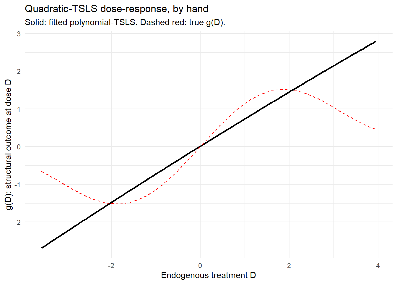
The figure makes the limitation visible: the quadratic-TSLS curve captures the overall concavity of \(g(D)\) in the middle of the support but cannot match the wiggle on the right tail, because a quadratic polynomial does not have enough degrees of freedom to fit a sinusoid. The diagnostic is twofold: the curve fails to bend back down in the right region, and the coefficient on \(D^2\) in the table is statistically significant, which means a linear-only specification would have been inadequate but the quadratic extension is also only partially adequate.
Increasing the polynomial degree improves the fit but quickly runs into the classical NPIV pathology: as the basis grows, the conditioning of the first-stage matrix degrades and the estimator becomes high-variance. The principled fix is data-driven choice of the basis dimension, which is exactly what the npiv package provides.
39.8.1.5.2 Production: npiv package with data-driven sieve
The npiv package by Christensen and collaborators implements the Newey and Powell (2003) sieve estimator with data-driven choice of the sieve dimension and uniform confidence bands obtained by a bootstrap procedure. The interface mirrors a standard regression call: pass the outcome, the endogenous treatment, the instrument, and an optional set of exogenous controls.
# install.packages("npiv")  # CRAN, Christensen and collaborators
library(npiv)

# Fit the NPIV estimator on the same simulated data.
# ucb_iter governs the uniform-confidence-band resampling;
# basis controls the sieve (B-splines by default).
fit <- npiv(
  Y        = Y,
  X        = D,        # endogenous variable
  W        = Z,        # instrument
  basis    = "bspline",
  ucb_iter = 1000
)
plot(fit, main = "NPIV dose-response of Y on endogenous D")
curve(sin(x) + 0.3 * x, add = TRUE, col = "red")
legend("topleft",
       legend = c("NPIV fit", "True g(d)"),
       col    = c("black", "red"),
       lty    = c(1, 1),
       bty    = "n")
The output of plot(fit) is the fitted structural function \(\hat{g}(d)\) on a fine grid of dose values, with a uniform 95% confidence band drawn around it. The companion summary(fit) returns the data-driven sieve dimension that was selected, the bootstrap iteration count, and a Wald-style test of the joint null \(g(d) = 0\) for all \(d\) in the band’s support. Reading the figure: the fitted curve should track the true \(g(d)\) across the support, including the right-tail wiggle that the quadratic-TSLS demo could not capture; the confidence band should be widest where the data are thinnest (typically the extreme tails) and narrowest where the instrument-induced variation in \(D\) is most informative.
Reading the demonstration and the production figures together is the right framing for the substantive payoff. The polynomial-TSLS line shows the failure mode of a fixed-basis approach: it cannot extrapolate beyond its functional form, and so it hides any feature of \(g(d)\) that lies outside the chosen polynomial family. The NPIV line shows the cure: the sieve dimension grows with the sample size, the data choose the basis, and the uniform band makes the inferential statement honestly. The cost is computational (the bootstrap is the bottleneck) and statistical (NPIV is data-hungry and degrades quickly when the instrument is weak), but for a continuous-treatment problem with enough data and a credible instrument, the NPIV deliverable is a structural function, not a single slope.
39.8.2 Granular IV and Structural Identification in the Global Oil Market
In empirical macroeconomics and international finance, distinguishing between aggregate and local (country-specific) shocks is often a powerful strategy for identification. Granular Instrumental Variables (GIV) exploit differences in local-level behavior to uncover aggregate relationships: micro-level deviations from the cross-sectional average serve as exogenous variation in identifying macroeconomic parameters. This section follows the structural application of Baumeister and Hamilton (2023) to the global oil market, building on the theoretical foundations laid by Gabaix and Koijen (2024).
It is useful to contrast GIV with the Bartik (shift-share) instrument. Bartik IVs combine a national exposure to aggregate shocks with weighted sums of industry-level shocks under common-shocks plus exogenous-weights assumptions; GIV instead aggregates idiosyncratic local shocks under an assumption that the granular shocks are independent.
39.8.2.1 Case Study: The Global Oil Market
Baumeister and Hamilton (2023) estimate oil supply and demand elasticities from 1973:M1 to 2023:M2 (excluding the COVID-19 period), using a structural system of equations to identify price elasticities. Producers are partitioned into \(n = 4\) groups (United States, Saudi Arabia, Russia, Rest of the World) and consumers into \(m = 4\) groups (United States, Japan, Europe, Rest of the World).
Let \(q_{it}\) be the growth rate of oil production in country \(i\) with world production share \(s_{qi}\), and \(c_{jt}\) the growth rate of oil consumption in country \(j\) with world consumption share \(s_{cj}\). Global growth rates are approximated by the weighted sums \(\sum_{i=1}^n s_{qi} q_{it}\) and \(\sum_{j=1}^m s_{cj} c_{jt}\).
Supply, demand, and inventory each have a structural representation. For supply,
\[q_{it} = \phi_{qi} p_t + \mathbf{b}_{qi}' \mathbf{x}_{t-1} + u_{qit} + u_{\chi it},\]
where \(\phi_{qi}\) is the short-run supply elasticity of country \(i\), \(\mathbf{x}_{t-1}\) collects lags of production, consumption, and the global oil price, \(u_{qit}\) is a structural supply shock, and \(u_{\chi it}\) is measurement error. In vector form \(\mathbf{q}_t = \boldsymbol{\phi}_q p_t + \mathbf{B}_q \mathbf{x}_{t-1} + \mathbf{u}_{qt} + \mathbf{u}_{\chi t}\). Demand is analogous:
\[c_{jt} = \phi_{cj} p_t + \mathbf{b}_{cj}' \mathbf{x}_{t-1} + u_{cjt} + u_{\psi jt},\]
with vector form \(\mathbf{c}_t = \boldsymbol{\phi}_c p_t + \mathbf{B}_c \mathbf{x}_{t-1} + \mathbf{u}_{ct} + \mathbf{u}_{\psi t}\). Inventories reconcile the difference between correctly measured global production and consumption,
\[v_t = \sum_{i=1}^n s_{qi} (q_{it} - u_{\chi it}) - \sum_{j=1}^m s_{cj} (c_{jt} - u_{\psi jt}),\]
with structural behavior \(v_t = \phi_v p_t + \mathbf{b}_v' \mathbf{x}_{t-1} + u_{vt}\). Combining supply, demand, and inventory yields the market-clearing identity that determines \(p_t\) endogenously:
\[\left( \mathbf{s}_q' \boldsymbol{\phi}_q - \mathbf{s}_c' \boldsymbol{\phi}_c - \phi_v \right) p_t = \left( \mathbf{s}_c' \mathbf{B}_c - \mathbf{s}_q' \mathbf{B}_q + \mathbf{b}_v' \right) \mathbf{x}_{t-1} + \mathbf{s}_c' \mathbf{u}_{ct} - \mathbf{s}_q' \mathbf{u}_{qt} + u_{vt}.\]
The system has \(n + m + 1\) equations for the \(n + m + 1\) endogenous variables \(\mathbf{q}_t, \mathbf{c}_t, p_t\) and is closed under structural assumptions about the shocks. Identification of \(\boldsymbol{\phi}_q\) and \(\boldsymbol{\phi}_c\) rests on cross-sectional variation in country-specific shocks, orthogonality of shocks across countries, independence of measurement errors from prices, and lagged variables in \(\mathbf{x}_{t-1}\) as instruments. The granular insight is that country-level production and consumption shocks are weakly correlated across countries, which makes the system well-suited for IV estimation; Baumeister and Hamilton (2023) estimate the full system by Full-Information Maximum Likelihood.
39.8.2.2 Demand-Side Worked Example: Constructing a Granular Instrument
Suppose the short-run demand elasticity is common across countries, \(\phi_{cj} = \phi_c\) for all \(j\). Decompose each country’s demand shock into a common global component \(f_{ct}\) and an idiosyncratic deviation \(\eta_{cjt}\):
\[c_{jt} = \phi_c p_t + \mathbf{b}_{cj}' \mathbf{x}_{t-1} + f_{ct} + \eta_{cjt} + u_{\psi jt}.\]
The unweighted cross-country average is
\[\bar{c}_t = \frac{1}{m} \sum_{j=1}^{m} c_{jt} = \phi_c p_t + \bar{\mathbf{b}}_c' \mathbf{x}_{t-1} + f_{ct} + \bar{\eta}_{ct} + \bar{u}_{\psi t}.\]
The country-specific deviation eliminates the price term and the common shock,
\[c_{jt} - \bar{c}_t = (\mathbf{b}_{cj}' - \bar{\mathbf{b}}_c') \mathbf{x}_{t-1} + (\eta_{cjt} - \bar{\eta}_{ct}) + (u_{\psi jt} - \bar{u}_{\psi t}),\]
so only idiosyncratic variation and measurement error remain. A more powerful instrument is constructed by combining country-specific deviations with the share-weighted consumption \(c_t = \sum_{j=1}^m s_{cj} c_{jt}\):
\[c_t - \bar{c}_t = \sum_{j=1}^{m} s_{cj} (c_{jt} - \bar{c}_t) = (\mathbf{b}_c' - \bar{\mathbf{b}}_c') \mathbf{x}_{t-1} + (\eta_{ct} - \bar{\eta}_{ct}) + (u_{\psi t} - \bar{u}_{\psi t}).\]
The difference between share-weighted and unweighted consumption is orthogonal to the endogenous price \(p_t\) (the price term cancels in both averages) and orthogonal to the common shock, leaving only idiosyncratic variation. Under the assumption that idiosyncratic demand shocks and measurement errors are uncorrelated with supply shocks, this difference is a valid and powerful instrument for the supply elasticity \(\phi_q\).
39.9 Econometric Foundations: Conditional Expectations, Projection, and Endogeneity
Before turning to the mechanics of instrumental variable estimation, it is worth establishing the conceptual scaffolding on which the entire method rests. Instrumental variables exist to solve a single problem: the parameter an economist wants to learn about is not, in general, the parameter that ordinary least squares recovers. Making that statement precise requires three ingredients, namely a clear definition of what it means for a parameter to be identified, a careful distinction between the conditional expectation function and the linear projection that least squares actually estimates, and a catalogue of the reasons the two can diverge. Once those pieces are in place, the role of an instrument follows almost mechanically. This section develops that foundation and connects it to the relevance, exogeneity, and rank conditions introduced in the main treatment of instrumental variables. The exposition follows the framework in Angrist and Pischke (2009) and the moment based development of identification associated with Hansen (1982).
39.9.1 Identification
A population parameter, written generically as \(\Theta\), is some functional of the distribution \(F\) of the observable data, say \(\Theta = g(F)\) for \(F\) in a class of admissible distributions \(\mathcal{F}\). The parameter is said to be identified when it both exists and is unique for every \(F \in \mathcal{F}\). Identification is a statement about the population, not about any particular sample. It asks whether, given perfect knowledge of the joint distribution of the observables, the parameter is pinned down at all. No amount of data can rescue a parameter that is not identified, and identification therefore logically precedes estimation.
Two examples make the idea concrete. The conditional mean \(E(Y \mid X = x)\) is identified whenever \(E|Y| < \infty\), because the distribution of the data determines it directly. The coefficients of a linear projection, introduced below, are identified as long as the second moment matrix \(E(\mathbf{X}'\mathbf{X})\) is nonsingular. In both cases the parameter is written as a function of moments of the observable random variables, and the equality sign in \(\Theta = g(F)\) carries the dual meaning of existence and uniqueness.
Consider the linear model \(Y = \beta_0 + \beta_1 X + U\). Suppose we impose the identification assumption that the error has conditional mean zero, \(E(U \mid X) = 0\), so that the conditional expectation is itself linear, \(E(Y \mid X) = \beta_0 + \beta_1 X\). The intercept is then identified as \(\beta_0 = E(Y \mid X = 0)\). The slope follows from the covariance,
\[ \text{Cov}(Y, X) = \text{Cov}(\beta_0, X) + \beta_1 \text{Var}(X) + \text{Cov}(U, X) = \beta_1 \text{Var}(X), \]
so that \(\beta_1 = \text{Cov}(Y, X) / \text{Var}(X)\) provided the additional condition \(\text{Var}(X) \neq 0\) holds, that is, provided \(X\) is not degenerate. Identification thus rests on two pieces: a stochastic restriction on the error and a support condition on the regressor. The first is the substantive assumption that may fail; the second is usually innocuous but still necessary.
It is useful to keep in mind a hierarchy of restrictions on the relationship between a regressor and an error term, ordered from weakest to strongest. The weakest is zero covariance, \(\text{Cov}(X, U) = 0\), which is equivalent to \(E(XU) = E(X)E(U)\) and is exactly what the linear projection imposes. Mean independence, \(E(U \mid X) = E(U)\), is stronger because it implies \(E(g(X) U) = E(g(X)) E(U)\) for any function \(g\), not merely for \(g\) linear. Full independence, \(U \perp X\), is strongest of all and implies \(E(g(X) h(U)) = E(g(X)) E(h(U))\) for arbitrary \(g\) and \(h\). The distinctions matter because different estimators and different interpretations require different rungs of this ladder, and much of the difficulty in applied work lies in arguing that a given rung is actually reached.
39.9.2 The Conditional Expectation Function
Most economic questions are questions about a conditional expectation function, written compactly as
\[ E(Y \mid W, \mathbf{C}), \]
where \(Y\) is the outcome, \(W\) is the variable of primary interest, and \(\mathbf{C}\) is a vector of control variables, some of which may be unobserved. We focus on the conditional expectation rather than the full conditional distribution \(F_{Y \mid W, \mathbf{C}}\) because the conditional mean is a single, tractable summary of the relationship that requires fewer assumptions to estimate credibly. Modeling the entire conditional distribution demands considerably more structure and tends to buy less internal validity in return, though conditional quantiles and other features of the distribution are sometimes of independent interest.
The conditional expectation function can be read in three quite different ways, and the reading determines which assumptions are required and what conclusions are licensed. Take the familiar wage equation,
\[ \ln(\text{wage}) = \beta_0 + \beta_1 \, \text{educ} + \beta_2 \, \text{exp} + \beta_3 \, \text{married} + U, \]
where \(U\) collects all unobserved factors affecting the wage offer. If we treat this as a structural or causal model, then the coefficients carry behavioral meaning and the equation should in principle be derivable from an underlying optimization problem; the cost is a heavy set of assumptions and restrictions needed to justify that derivation. If we treat it as a conditional expectation function, then the relevant worry is whether \(E(U \mid \mathbf{X}) = 0\) actually holds, since unobserved factors lurking in \(U\) may well be correlated with schooling or experience. If we treat it merely as a linear projection, then there is nothing to worry about at all, because the projection always exists, but the interpretation becomes purely descriptive rather than causal.
Specifying a conditional expectation also requires specifying the population of interest, since the same conditioning variables can describe very different populations. A poorly chosen population is one in which the variable of interest exhibits little or no variation, leaving nothing for the data to identify.
A model for the conditional expectation can be classified along several dimensions. A specification such as \(E(Y \mid X_1, X_2) = \beta_0 + \beta_1 X_1 + \beta_2 X_2\) is linear in the variables, because it is a linear combination of \((1, X_1, X_2)\), and adding a term like \(\beta_3 X_2^2\) or \(\beta_3 X_1 X_2\) would violate linearity in variables while remaining linear in parameters. It is linear in the parameters because it is a linear combination of \((\beta_0, \beta_1, \beta_2)\), and a term like \(X_1^{\gamma}\) would violate that. It is parametric because it involves a finite number of unknown parameters rather than an unknown function; replacing \(\beta_2 X_2\) with an unknown \(g(X_2)\) would make it nonparametric. A semiparametric model combines a finite dimensional parameter of interest with an infinite dimensional nuisance component. These are modeling choices rather than properties of the data: the very same equation \(Y = \mathbf{X}\boldsymbol{\beta} + U\) can be approached as parametric, semiparametric, or nonparametric depending on what one is willing to assume.
39.9.3 Linear Projection
Most of the examples above quietly imposed linearity on the conditional expectation function, an assumption that need not hold. The linear projection provides a way to obtain an estimable equation without that assumption, at the price of a weaker interpretation. Let \(\mathbf{X} = (X_1, \dots, X_k)\) be a \(1 \times k\) vector whose \(k \times k\) variance matrix is positive definite. The linear projection of \(Y\) on a constant and \(\mathbf{X}\) then exists and is unique,
\[ L(Y \mid 1, \mathbf{X}) = \gamma_0 + \gamma_1 X_1 + \dots + \gamma_k X_k, \]
with slope coefficients and intercept defined by
\[ \boldsymbol{\gamma} = [\text{Var}(\mathbf{X})]^{-1} \text{Cov}(\mathbf{X}, Y), \qquad \gamma_0 = E(Y) - E(\mathbf{X}) \boldsymbol{\gamma}. \]
These objects are functions of population moments and are therefore identified and estimable. Equivalently, we may write \(Y = \gamma_0 + \gamma_1 X_1 + \dots + \gamma_k X_k + U\), where the projection error satisfies, by construction, \(E(U) = 0\) and \(\text{Cov}(X_j, U) = 0\) for every \(j\). It is essential to recognize what these properties do not say. Zero covariance does not imply that \(U\) is independent of \(\mathbf{X}\), nor even that it is mean independent. The projection error can depend on the regressors in arbitrarily rich ways so long as it is linearly uncorrelated with each of them.
The linear projection has several properties that explain why it is the natural object of least squares estimation. First, the projection coefficient is the minimum mean square linear predictor, since it solves \(\min_{b_0, \mathbf{b}} E[(Y - b_0 - \mathbf{X}\mathbf{b})^2]\). Second, the conditional expectation function is the minimum mean square predictor among all functions, since it solves \(\min_{g} E[(Y - g(\mathbf{X}))^2]\). Third, when the conditional expectation happens to be linear in \(\mathbf{X}\), the projection coincides exactly with the conditional expectation. Fourth, and most usefully, even when the conditional expectation is not linear, the projection is the best linear approximation to it in the mean square sense.
The last claim deserves a short proof, because it is what justifies reporting a linear regression even when one does not believe the truth is linear. The best linear approximation to the conditional expectation solves \(\min_{b_0, \mathbf{b}} E[(E(Y \mid \mathbf{X}) - b_0 - \mathbf{X}\mathbf{b})^2]\), whereas the projection solves \(\min_{b_0, \mathbf{b}} E[(Y - b_0 - \mathbf{X}\mathbf{b})^2]\). For any \(b_0\) and \(\mathbf{b}\), add and subtract the conditional expectation inside the square,
\[ \begin{aligned} E[(Y - b_0 - \mathbf{X}\mathbf{b})^2] &= E[(Y - E(Y \mid \mathbf{X}))^2] + E[(E(Y \mid \mathbf{X}) - b_0 - \mathbf{X}\mathbf{b})^2] \\ &\quad + 2 E[(Y - E(Y \mid \mathbf{X}))(E(Y \mid \mathbf{X}) - b_0 - \mathbf{X}\mathbf{b})]. \end{aligned} \]
The cross term vanishes by the law of iterated expectations, since conditioning on \(\mathbf{X}\) leaves \(E(Y \mid \mathbf{X}) - b_0 - \mathbf{X}\mathbf{b}\) fixed while \(E(Y - E(Y \mid \mathbf{X}) \mid \mathbf{X}) = 0\). Because the first term does not depend on the choice of \(b_0\) and \(\mathbf{b}\), the two minimization problems share the same argument minimizer,
\[ \arg\min_{b_0, \mathbf{b}} E[(Y - b_0 - \mathbf{X}\mathbf{b})^2] = \arg\min_{b_0, \mathbf{b}} E[(E(Y \mid \mathbf{X}) - b_0 - \mathbf{X}\mathbf{b})^2]. \]
The projection coefficient is therefore the best mean square linear approximation to the conditional expectation function, which is precisely why least squares remains informative as a descriptive device even when the causal model is nonlinear.
The decomposition is easy to see in a small simulation. The conditional expectation below is genuinely nonlinear in \(x\), yet the population projection coefficient recovered by least squares matches the slope obtained by regressing the true conditional mean on \(x\), confirming that the projection is approximating \(E(Y \mid X)\) rather than \(Y\) itself.
set.seed(123)
n <- 100000
x <- runif(n, -2, 2)
cef <- 1 + 0.8 * x + 0.5 * x^2          # nonlinear conditional expectation
y <- cef + rnorm(n)                     # outcome adds mean-zero noise

# projection of the outcome on (1, x)
coef_outcome <- coef(lm(y ~ x))["x"]
# projection of the conditional expectation on (1, x)
coef_cef <- coef(lm(cef ~ x))["x"]

round(c(projection_on_Y = coef_outcome,
        projection_on_CEF = coef_cef), 4)
#>   projection_on_Y.x projection_on_CEF.x
#>              0.7979              0.8005
The two slopes agree up to sampling noise, illustrating that the linear projection of \(Y\) is the best linear approximation to the conditional expectation function and not merely a summary of the raw outcome.
39.9.4 Endogeneity in the Linear Model
Now suppose the object of interest is genuinely structural. Write the population model as linear in parameters,
\[ Y = \beta_0 + \beta_1 X_1 + \dots + \beta_k X_k + U = \mathbf{X}\boldsymbol{\beta} + U, \]
where \(\mathbf{X}\) stacks a constant with the regressors and the \(\beta_j\) are the behavioral parameters we wish to estimate. Ordinary least squares is consistent for these parameters when the orthogonality condition \(E(\mathbf{X}' U) = 0\) holds. A regressor \(X_j\) is called endogenous precisely when this condition fails through \(\text{Cov}(X_j, U) \neq 0\). When that happens, the structural coefficient \(\beta_j\) cannot coincide with the linear projection coefficient, even though the latter always exists and is always estimable. This is the formal version of the warning that correlation, which the projection captures, is not the same as causation, which is what the structural coefficient is meant to represent.
There are three classic sources of endogeneity, each of which recurs throughout applied work and each of which motivates the instrumental variable solution. The first is omitted variables, where a determinant of the outcome that is correlated with an included regressor is left out of the equation, often because it is unobservable. The second is measurement error, where the analyst would like to study the effect of a true variable \(X_k^{*}\) but observes only an imperfect proxy \(X_k\), or would like to explain a true outcome \(Y^{*}\) but observes only a noisy measure \(Y\). The third is simultaneity, where outcome and regressor are jointly determined, as in a market where price depends on quantity demanded while quantity demanded depends on price; this case is central to general equilibrium and supply and demand systems and was the setting in which instrumental variables were first developed (Wright 1928).
The omitted variable case repays a careful look because it shows exactly how the structural parameter and the projection parameter separate. Suppose the true causal model is
\[ Y = \beta_0 + \beta_1 X + \gamma Q + V, \qquad E(V \mid X, Q) = 0, \]
so that \(\beta_1\) is the effect of \(X\) on \(Y\) holding the omitted variable \(Q\) fixed. If \(Q\) is dropped, the working error becomes \(U = \gamma Q + V\), and the orthogonality of \(X\) with \(U\) reduces to
\[ \text{Cov}(X, U) = \gamma \, \text{Cov}(X, Q), \]
which is nonzero whenever \(X\) is correlated with \(Q\) and \(Q\) genuinely affects \(Y\), that is, \(\gamma \neq 0\). To see what least squares then estimates, project the omitted variable on the included regressor, \(Q = \delta_0 + \delta_1 X + R\), with \(\delta_1 = \text{Cov}(X, Q)/\text{Var}(X)\) and \(\text{Cov}(X, R) = 0\) by construction. Substituting,
\[ Y = (\beta_0 + \gamma \delta_0) + (\beta_1 + \gamma \delta_1) X + (\gamma R + V), \]
and the composite error \(\gamma R + V\) now satisfies both projection conditions. Least squares is therefore consistent for the projection slope \(\beta_1 + \gamma \delta_1\), so that
\[ \text{plim}\, \hat{\beta}_1 = \beta_1 + \gamma \frac{\text{Cov}(X, Q)}{\text{Var}(X)}. \]
The inconsistency, \(\text{plim}\, \hat{\beta}_1 - \beta_1 = \gamma \, \text{Cov}(X, Q)/\text{Var}(X)\), is the omitted variable bias, and its sign is the product of two pieces: the direction of the correlation between the included regressor and the omitted variable, and the direction of the omitted variable’s effect on the outcome. Both must be nonzero and their signs jointly determine whether least squares overstates or understates the causal effect.
39.9.5 Instrumental Variables and the Method of Moments
Return to the simplest endogenous model, \(Y = \beta_0 + \beta_1 X + U\) with \(\text{Cov}(X, U) \neq 0\). The identification problem is that the observed covariation between \(X\) and \(Y\) blends two distinct sources of variation,
\[ \text{Cov}(X, Y) = \beta_1 \text{Var}(X) + \text{Cov}(X, U), \]
so that the projection slope \(\text{Cov}(X, Y)/\text{Var}(X)\) equals \(\beta_1\) plus a bias term \(\text{Cov}(X, U)/\text{Var}(X)\) that does not vanish. Variation in \(X\) that is correlated with \(U\) contaminates the comparison, and no reweighting of the existing data can separate the two.
The instrumental variable solution is to bring in a new source of variation through an instrument \(Z\) that satisfies two conditions. The relevance condition, \(\text{Cov}(Z, X) \neq 0\), requires that the instrument actually move the endogenous regressor and is testable from the data. The exogeneity condition, or exclusion restriction, \(\text{Cov}(Z, U) = 0\), requires that the instrument be uncorrelated with the structural error and is fundamentally a matter of judgment that cannot be verified directly. The canonical illustration is the use of quarter of birth as an instrument for years of schooling in studies of the returns to education (Angrist and Krueger 1991), though later work questioning the strength of the instrument and documenting systematic differences in family background across birth seasons is a reminder that the relevance and exclusion conditions are never beyond challenge (Bound et al. 1995; Buckles and Hungerman 2013).
To see why a valid instrument solves the problem, project the endogenous regressor on the instrument, \(X = \delta_0 + \theta Z + R\), splitting \(X\) into an exogenous part driven by \(Z\) and a residual part \(R\) with \(E(R) = 0\) and \(\text{Cov}(Z, R) = 0\). The endogeneity of \(X\) then lives entirely in the residual,
\[ \text{Cov}(X, U) = \theta \, \text{Cov}(Z, U) + \text{Cov}(R, U) = \text{Cov}(R, U), \]
because the instrument is exogenous. Using only the \(Z\) driven part of \(X\) therefore strips out the contaminated variation and isolates the causal effect.
The argument generalizes cleanly to the multiple regressor case and connects directly to the method of moments. Write the model as \(Y = \mathbf{X}\boldsymbol{\beta} + U\) with a single endogenous regressor \(X_k\), so that \(\text{Cov}(X_k, U) \neq 0\) while the remaining regressors are exogenous. It is worth stressing that there is no such thing as an OLS model as opposed to an IV model; least squares and instrumental variables are competing estimation strategies for the same underlying linear model. Given an external instrument \(Z_k\) for \(X_k\), build the instrument vector \(\mathbf{Z} = (1, X_2, \dots, X_{k-1}, Z_k)\) alongside the regressor vector \(\mathbf{X} = (1, X_2, \dots, X_{k-1}, X_k)\), both \(1 \times k\), in which every exogenous regressor instruments for itself. Two assumptions then drive identification. Exogeneity becomes \(E(\mathbf{Z}' U) = 0\). The rank condition, which replaces simple relevance in the vector setting, is \(\text{rank}\,[E(\mathbf{Z}' \mathbf{X})] = k\), equivalently the requirement that \(E(\mathbf{Z}' \mathbf{X})\) be invertible.
The exogeneity assumption is best understood as a moment condition. Substituting the model,
\[ E(\mathbf{Z}' U) = 0 \quad \Longleftrightarrow \quad E(\mathbf{Z}'(Y - \mathbf{X}\boldsymbol{\beta})) = 0, \]
expresses the expectation of a known function of observables and unknown parameters as equal to zero. Moment conditions of exactly this form are the foundation of generalized method of moments estimation (Hansen 1982), and the overidentification tests associated with it descend from the early work on testing instrument validity in simultaneous systems (Sargan 1958). The rank condition is the matrix counterpart of relevance combined with the absence of perfect multicollinearity. Concretely, assuming no perfect collinearity among \(1, X_2, \dots, X_{k-1}\), the rank condition holds if and only if the coefficient \(\theta\) on the instrument in the first stage projection
\[ L(X_k \mid 1, X_2, \dots, X_{k-1}, Z_k) = \delta_1 + \delta_2 X_2 + \dots + \delta_{k-1} X_{k-1} + \theta Z_k \]
is nonzero. In words, after partialling out the other exogenous regressors, the instrument must still be correlated with the endogenous variable, and because this is a statement about a regression coefficient it is testable.
Under exogeneity and the rank condition the instrument identifies the structural parameter. Premultiply the model by \(\mathbf{Z}'\) and take expectations,
\[ E(\mathbf{Z}' Y) = E(\mathbf{Z}' \mathbf{X}) \boldsymbol{\beta} + E(\mathbf{Z}' U) = E(\mathbf{Z}' \mathbf{X}) \boldsymbol{\beta}, \]
and invert the now nonsingular cross moment matrix to obtain
\[ \boldsymbol{\beta} = [E(\mathbf{Z}' \mathbf{X})]^{-1} E(\mathbf{Z}' Y). \]
The sample analogue replaces population moments with their empirical counterparts, yielding the instrumental variable estimator
\[ \hat{\boldsymbol{\beta}}_{IV} = (\mathbf{Z}' \mathbf{X})^{-1} \mathbf{Z}' \mathbf{Y} = \boldsymbol{\beta} + (\mathbf{Z}' \mathbf{X})^{-1} \mathbf{Z}' \mathbf{U}. \]
Consistency follows because the second term converges to zero in probability under exogeneity, while the rank condition guarantees that the inverse exists in large samples. The interpretation of the resulting estimand, the local average treatment effect that applies to the compliers whose treatment is shifted by the instrument, is developed in the identification framework for instrumental variables and in the foundational treatment of Imbens and Angrist (1994). A practical caution carries over from the structural setting: if any of the variables treated as controls are themselves endogenous, the resulting inconsistency contaminates every coefficient in \(\hat{\boldsymbol{\beta}}_{IV}\), not merely the coefficient on the variable for which an instrument was sought.
The same logic can be visualized in a short simulation that contrasts the inconsistent least squares estimator with the consistent instrumental variable estimator when the regressor is endogenous and a valid instrument is available.
set.seed(456)
n <- 200000
z <- rnorm(n)                       # exogenous instrument
u <- rnorm(n)                       # structural error
x <- 0.7 * z + u + rnorm(n)         # x is correlated with u (endogenous)
beta_true <- 2
y <- 1 + beta_true * x + u          # u enters both x and y

ols <- coef(lm(y ~ x))["x"]                 # biased by Cov(x, u)
# IV via the ratio of covariances in the just-identified case
iv  <- cov(z, y) / cov(z, x)

round(c(true = beta_true, ols = ols, iv = iv), 4)
#>   true  ols.x     iv
#> 2.0000 2.4010 1.9983
Least squares is pulled away from the true value of two by the correlation between \(x\) and the error, whereas the instrumental variable estimator, formed here as the ratio \(\text{Cov}(Z, Y)/\text{Cov}(Z, X)\) in the just identified case, recovers the structural parameter up to sampling noise. This is the payoff of the entire construction: by importing exogenous variation through a valid instrument, the method of moments identifies the structural coefficient that ordinary least squares cannot.
39.9.7 Recentered Instrumental Variables
Modern empirical work routinely uses formula instruments: variables that combine exogenous shocks with predetermined characteristics through a known function. The shift-share instrument is the leading example, but the class is much broader, including market-access measures, transportation upgrades, simulated eligibility scores, and centralized assignment indices. Borusyak and Hull (2023) show that whenever exposure to exogenous shocks is itself nonrandom, even unbiased shocks can generate omitted-variable bias in the constructed instrument. Their Recentered Instrumental Variable (RIV) framework removes this bias by subtracting each unit’s expected exposure under a credible counterfactual shock distribution.
The settings where RIV is useful include linear SSIV (Autor et al. 2013; Borusyak et al. 2022); nonlinear SSIV (Boustan et al. 2013; Chodorow-Reich and Wieland 2020; Derenoncourt 2022); centralized school-assignment mechanisms (Abdulkadiroğlu et al. 2017; Angrist et al. 2020); model-implied optimal IVs (Adao, Arkolakis, et al. 2019); weather instruments (Madestam et al. 2013); and mass-media exposure via free-space propagation (Olken 2009; Yanagizawa-Drott 2014).
39.9.7.1 Motivating Examples
Market access from China’s high-speed rail. Suppose we want to estimate how transportation infrastructure affects land value via market access:
\[\Delta \log V_i = \beta\, \Delta \log MA_i + \varepsilon_i, \qquad MA_{it} = \sum_k \tau(g_t, \text{loc}_i, \text{loc}_k)^{-1}\, \text{pop}_k,\]
where \(g_t\) is the road network at time \(t\), \(\tau\) is a travel-cost function, and \(\text{pop}_k\) is destination population. Even if construction is randomized, \(MA_i\) is not, because the transformation through geography and population introduces nonrandom exposure. Periphery regions hit by sea-level rise or differential regional growth trends may correlate with where market access happens to grow. The realized \(\Delta MA_i\) is therefore endogenous as an instrument for any outcome that varies systematically with geography.
Medicaid eligibility. When state policies \(g_s\) are assumed randomly assigned across states but individual eligibility \(x_i\) depends jointly on \(g_s\) and predetermined demographics (income, age, family composition), even a state-level expansion dummy is an inefficient instrument for individual eligibility. The simulated-eligibility instrument of Currie and Gruber (1996) instruments using an average eligibility rate computed for a fixed reference sample, but this discards heterogeneity in how strongly different demographics respond to a given policy expansion.
In both cases, the construction \(z_i = f_i(g, w)\) is a known formula in exogenous shocks \(g\) and predetermined characteristics \(w\), but the formula itself induces structured variation that need not be exogenous to the outcome.
39.9.7.2 Formal Framework
We estimate
\[y_i = \beta x_i + \varepsilon_i, \qquad i = 1, \dots, N,\]
with treatment \(x_i\), unobserved error \(\varepsilon_i\), and a candidate instrument constructed as
\[z_i = f_i(g, w),\]
where \(g = (g_1, \dots, g_K)\) is a vector of exogenous shocks, \(w\) collects observed predetermined characteristics, and \(f_i\) is a known formula. The formula is general: it nests linear SSIV (\(f_i(g, w) = \sum_k s_{ik} g_k\)), reduced-form designs (\(x_i = z_i\)), and nonlinear or interactive constructions.
Even when \(g \perp\!\!\!\perp \varepsilon_i \mid w\), the constructed instrument \(z_i\) need not satisfy \(z_i \perp\!\!\!\perp \varepsilon_i\). This is because \(f_i(g, w)\) may systematically assign larger values of \(z_i\) to units with particular, potentially unobserved characteristics, generating an omitted-variable bias of the form
\[\mathbb{E}\!\left[\frac{1}{N}\sum_i z_i \varepsilon_i\right] = \mathbb{E}\!\left[\frac{1}{N}\sum_i \mu_i \varepsilon_i\right] \ne 0,\]
where \(\mu_i = \mathbb{E}_{g' \sim G(\cdot\mid w)}[f_i(g', w)]\) is each unit’s expected instrument under the known shock distribution.
39.9.7.3 Why Recentering Works
Define the recentered instrument
\[\tilde z_i = z_i - \mu_i.\]
By construction \(\mathbb{E}[\tilde z_i \mid w] = 0\), and under shock exogeneity,
\[\mathbb{E}\!\left[\frac{1}{N}\sum_i \tilde z_i \varepsilon_i\right] = 0,\]
so \(\tilde z_i\) is a valid instrument for identifying \(\beta\). An algebraically equivalent procedure is to control for \(\mu_i\) directly in the second stage and use the original \(z_i\) as the instrument, by Frisch-Waugh-Lovell. The control-function variant can be more efficient when treatment effects are heterogeneous.
For the linear SSIV special case, the expected instrument simplifies. If \(g_k\) is exogenous conditional on shares, \(\mathbb{E}[g_k \mid \mathbf{s}] = \gamma\), then \(\mu_i = \gamma S_i\) where \(S_i = \sum_k s_{ik}\). Controlling for the sum of shares \(S_i\) is then sufficient. If \(g_k\) is exogenous only conditional on shock-level covariates \(q_k\), with \(\mathbb{E}[g_k \mid \mathbf{s}, \mathbf{q}] = q_k'\gamma\), then \(\mu_i = \gamma'\sum_k s_{ik} q_k\), and controlling for the share-weighted average of \(q_k\) suffices. This recovers, from a single recentering identity, the leave-one-out and exposure-weighted control structure that the recent SSIV literature has converged on.
39.9.7.4 Assumptions and the Shock Assignment Process
To compute \(\mu_i\) and identify causal effects, we need two assumptions on the shock assignment process:
- Shock exogeneity: \(g \perp \varepsilon \mid w\). Satisfied when shocks arise from randomized assignment (lotteries, RCTs), natural variation (weather, seismic activity), or plausibly exogenous policy mechanisms.
- Known conditional shock distribution: \(G(g \mid w)\) is known, either from the randomization protocol or from a design-based permutation distribution over plausible counterfactual assignments.
These yield the expected instrument
\[\mu_i = \int f_i(g, w)\, dG(g \mid w),\]
which can be evaluated analytically in simple cases (linear SSIV) and by simulation in complex ones.
39.9.7.5 Estimation Procedure
The recipe is:
- Define the instrument formula: \(z_i = f_i(g, w)\).
- Specify the assignment process: commit to a credible distribution \(G(g \mid w)\).
- Generate counterfactual shocks: simulate \(S\) draws \(g^{(s)} \sim G(g \mid w)\).
- Compute the expected instrument: \(\mu_i = S^{-1}\sum_{s=1}^S f_i(g^{(s)}, w)\).
- Recenter: \(\tilde z_i = z_i - \mu_i\).
- Estimate the IV regression using \(\tilde z_i\) as instrument for \(x_i\).
The alternative control-function form replaces step 5 with including \(\mu_i\) as a covariate:
\[y_i = \beta x_i + \lambda \mu_i + u_i, \qquad z_i \text{ instruments for } x_i.\]
Number of simulation draws \(S\) is set so that simulation noise in \(\mu_i\) is negligible relative to the residual scale. Several thousand draws is typical; the cost is embarrassingly parallel.
39.9.7.6 Properties: Consistency, Inference, Optimality
Consistency. The RIV estimator is consistent under mild regularity: sufficient variation in shocks across units, the known shock assignment process, and finite second moments. Crucially, no assumption is required on the correlation structure of \(\varepsilon_i\). This makes the method robust to complex spatial or network dependence, which is a significant practical advantage in spatial and platform-economics applications.
Inference. Standard errors based on the usual CLT may be invalid when units exposed to shared shocks have correlated residuals. Borusyak and Hull (2023) advocate randomization inference: define a test statistic based on recentered residuals, simulate its distribution under resampled \(g^* \sim G(\cdot \mid w)\), and construct confidence intervals by test inversion. Under constant treatment effects, this yields exact finite-sample inference conditional on \(w\).
Optimality. Among all instruments of the form \(f_i(g, w)\), Borusyak and Hull (2023) characterize an asymptotically efficient recentered instrument, generalizing the optimal-weighting result of GMM to structured IV settings.
39.9.7.7 Extensions
- Heterogeneous treatment effects. When \(\beta_i\) varies, \(\tilde z_i\) identifies a convex average of \(\beta_i\) under first-stage monotonicity, analogous to LATE.
- Nonlinear treatments. The framework accommodates \(x_i = h_i(g, w, u)\) with unobserved component \(u\). The candidate instrument \(z_i = h_i(g, w, 0)\) is recentered over \(g\) to purge bias from nonrandom exposure.
- Propensity-score analogy. RIV is structurally similar to propensity-score adjustment but applies to formula treatments rather than binary ones, and avoids estimating a high-dimensional propensity function.
39.9.7.8 Application: Market Access from China’s High-Speed Rail
Borusyak and Hull (2023) apply the recentering method to the effect of market-access growth from China’s high-speed rail (HSR) network on prefectural employment. Between 2008 and 2016, 83 HSR lines were built connecting major cities; an additional 66 lines were planned but not built by 2016. The goal is to estimate the causal effect of increased market access on employment growth across 274 prefectures between 2007 and 2016.
Market access for prefecture \(i\) in year \(t\) is
\[MA_{it} = \sum_k \exp(-0.02 \tau_{ikt})\, p_{k,2000},\]
with HSR-affected travel time \(\tau_{ikt}\) from Zheng and Kahn (2013) and year-2000 population \(p_{k,2000}\). Raw comparisons across regions with different \(\Delta MA\) confound HSR effects with regional trends, geography, and historical investment patterns. Controlling for province fixed effects helps but does not remove the structural problem: \(MA\) is constructed via a travel-cost model, and there is no experimental analog to benchmark the controls.
Earlier work attacks this through alternative natural experiments (Bartelme et al. 2018; Donaldson 2018). Borusyak and Hull (2023) instead isolate the plausibly exogenous component of timing of construction among observably similar lines. Assume the set of lines (built and unbuilt) was fixed as of 2019. Randomly reshuffle which 83 of these were built by 2016, maintaining the same number and connectivity structure. Use these reshuffled draws to estimate the expected market-access growth \(\mu_i\) under random assignment, and form
\[\tilde z_i = \Delta \log MA_i - \mu_i.\]
The recentered instrument removes systematic variation correlated with geography or development trends, isolating the HSR-driven component of market-access growth.
39.9.7.9 Application: Medicaid Expansion Efficiency
The second application revisits the 2014 Medicaid expansion. Of 43 states with initially low coverage, 19 expanded eligibility to 138% of the federal poverty line. Expansion decisions are treated as as-good-as-random among states with same-party governors. Household demographics and pre-2014 policy environments are not randomly assigned.
Two estimators are valid under the same identification assumptions:
- Simulated IV (Currie and Gruber 1996): use a state-level expansion dummy as the instrument for individual-level eligibility, with simulated eligibility computed for a fixed reference sample.
- Recentered IV (Borusyak and Hull 2023): predict eligibility \(x_i\) from state expansion status and predetermined demographics, then recenter using \(\mu_i = \mathbb{E}[x_i \mid \text{random expansion}]\).
The recentered IV estimator delivers standard errors roughly three times smaller than the simulated IV. The efficiency gain comes from exploiting within-state variation across heterogeneous households, which the simulated-eligibility approach throws away by computing eligibility for a single fixed reference sample.
39.9.7.10 Practical Considerations
The main costs and design choices:
- Computational burden. Simulating \(\mu_i\) requires repeated evaluation of \(f_i\) across counterfactual shocks. This is parallelizable and rarely the binding constraint.
- Choice of counterfactual distribution. The credibility of \(G(g \mid w)\) is the design’s load-bearing assumption. Permutation distributions are transparent; structural distributions can be more powerful but require their own defense. Report sensitivity to the choice.
- Falsification. Test balance of \(\tilde z_i\) against predetermined covariates and inspect pre-trends. Report results under alternative reshuffling strategies as robustness checks.
- Layered controls. Including predetermined controls after recentering can improve efficiency without compromising identification. Using both the control-function form and the recentered instrument is a form of double robustness.
Recentered IV is most valuable in applied settings where treatments arise from structural formulas, geographic interactions, or networked exposure, and where the standard IV assumption that the constructed instrument is itself exogenous would be implausible.
39.9.8 Decision-Maker IV
Examiner designs, judge IV designs, and leniency IV refer to a family of instrumental variable strategies that exploit quasi-random assignment of decision-makers (such as judges or examiners) to observational units. These designs are used to identify causal effects in settings where controlled experiments are not feasible.
The examiner/judge IV design is an approach where the instrument is the identity or behavior of an assigned decision-maker (an “examiner” or a judge). The classic setup arises in courts: cases are typically assigned to judges in a manner that is as good as random (often conditional on timing or location), and different judges have systematically different propensities to rule harshly or leniently. This means that, purely by the luck of the draw, otherwise-similar individuals may receive different treatments (e.g. a longer vs. shorter sentence) depending on which judge they happen to get. In such a design, the judge assignment (or a function of it) serves as an instrumental variable for the treatment of interest (like sentence length). The key insight is that who the examiner/judge is can be treated as an exogenous shock that influences the treatment but is (ideally) unrelated to the person’s own characteristics.
The term judge IV design specifically refers to using judges in legal settings as instruments. This approach rose to prominence through studies of the criminal justice system; a well-known early example is Kling (2006), who used randomly assigned judges to instrument for incarceration length when studying its effect on later earnings. More generally, the literature often calls this the “judge leniency” design, because it leverages differences in judges’ leniency/harshness. Importantly, the same idea extends beyond literal judges. Examiners in various administrative or medical contexts can play an analogous role. For instance, bureaucrats evaluating benefit claims, patent examiners reviewing applications, or physicians making discretionary treatment decisions can all act like “judges” whose assignment is as-good-as-random and whose leniency varies. In these non-court contexts, researchers sometimes use the term examiner design as a more general label, but it is essentially the same IV strategy. In summary, whether we say examiner design, judge IV, or judge leniency IV, we are usually referring to the same identification strategy: using the quasi-random assignment of a decision-maker with varying tendencies as an instrument.
How the design is structured: in practice, one can implement this IV in a couple of ways. One method is to include dummy variables for each judge/examiner as instruments (since each judge is a distinct source of variation). Another common approach is to construct a leniency measure for each decision-maker (for example, the judge’s historical rate of granting the treatment) and use that as a single continuous instrument. The latter approach (using a summary measure of leniency) is popular because it reduces dimensionality and mitigates weak-instrument concerns when there are many judges. For instance, instead of having 50 separate judge dummies, one can calculate each judge’s leave-one-out approval or sentencing rate and use that number as the instrument. This “leave-one-out” or jackknife approach ensures the measure for each judge is calculated excluding the case in question (avoiding mechanical endogeneity). Overall, the examiner/judge IV design turns the naturally occurring randomness in examiner assignment into a source of exogenous variation: who you were randomly assigned to becomes the instrument for the treatment you received.
39.9.8.1 Achieving Identification with a Leniency IV
The examiner/judge design is a powerful way to achieve identification in observational data. It rests on the core requirements for a valid instrumental variable:
-
Quasi-Random Assignment (Exogeneity): because examiners or judges are assigned to cases essentially at random (often by rotation, scheduling, or lottery), the particular decision-maker an individual gets is independent of that individual’s characteristics. This approximates the randomness of an experiment. As long as assignment is truly random (or as-good-as-random after conditioning on any known factors like time or location), the examiner identity is uncorrelated with unobserved confounders. In other words, which judge you draw should have no direct bearing on your outcome except through the judge’s decision. This satisfies the exogeneity condition for an IV.
Discretion over a binary treatment: each decision maker has discretionary authority over a treatment variable \(D_i\), typically binary (e.g., pretrial release vs. detention).
Heterogeneity in behavior: decision makers differ systematically in their propensity to assign treatment, allowing us to use these differences as instrumental variation.
Instrument Relevance: different examiners have different propensities to deliver the treatment. Some judges are more severe (more likely to incarcerate or give long sentences), while others are more lenient; some doctors are more likely to prescribe an intensive treatment, etc. This translates into substantial variation in the probability of treatment based solely on who the case was assigned to. For example, in the patent context, being assigned a lenient patent examiner vs. a strict one can significantly change the probability of a patent grant (Farre-Mensa et al. 2020).
Exclusion Restriction: the IV assumption is that the assigned examiner affects the outcome only through the treatment itself. In a judge design, this means the “type of judge you are assigned” should impact the defendant’s future outcomes solely via the judge’s decision (e.g. incarceration or release), not through any other channel. For instance, a harsh judge might send you to prison while a lenient judge might not, and that difference can affect your future, but we assume that it’s only the incarceration that matters for your future outcome, not any direct effect of interacting with a harsh vs. nice judge per se. This exclusion restriction is more plausible when the decision-maker has no direct interaction with the individual beyond making the decision. Researchers take care to argue that conditional on the controls and the treatment itself, the identity of the examiner has no independent effect on outcomes. If these conditions (relevance and exogeneity/exclusion) hold, then the variation in treatment induced by examiner assignment can be used to consistently estimate the causal effect of the treatment.
By meeting these conditions, examiner/judge IV designs create a natural experiment. Essentially, they compare outcomes between individuals who, by random luck, received different treatment assignments (e.g. one was incarcerated, another not) due to differing examiner leniency, despite those individuals being comparable in expectation. This helps isolate the causal impact of the treatment from confounding factors. Notably, the estimates from such designs often correspond to a local average treatment effect (LATE) for those cases whose treatment status is swayed by the examiner’s leniency, for example, the “marginal” defendants who would be incarcerated by a strict judge but released by a lenient judge. In sum, these designs allow researchers to mimic a randomized experiment within observational data by leveraging institutional randomness (who gets assigned to whom) as an instrument.
39.9.8.2 Leniency IV: Clarifying the Terminology
The term leniency IV refers to this same instrumental variable strategy, emphasizing the role of the examiner’s leniency (or strictness). In many studies, the instrument is literally a measure of how lenient the assigned judge or examiner tends to be. For example, in a Social Security Disability study, researchers “exploit variation in examiners’ allowance rates as an instrument for benefit receipt.” (Maestas et al. 2013). Here, an examiner’s allowance rate (the fraction of cases they approve) is a direct quantification of their leniency, and this serves as the instrumental variable. Similarly, one can define a judge’s leniency as the percentage of past defendants that judge jailed or the average sentence length they give, and use that as the IV. The phrase “leniency design” or leniency instrument simply underscores that it’s the lenient vs. strict tendencies of the decision-maker that provide the exogenous variation.
A leniency IV design typically involves constructing an instrument like “the leave-out mean decision rate of the assigned examiner.” This could be, for instance, the fraction of previous similar cases that the examiner approved (excluding the current case). That number captures how lenient or strict they generally are. Because assignment is random, some individuals get a high-leniency examiner and others a low-leniency examiner, creating exogenous variation in treatment. By comparing outcomes across these, one can identify the causal effect of the treatment. The term “leniency” highlights that it’s the discretionary toughness of the examiner that we’re leveraging.
39.9.8.3 Examples in Economics
Many influential studies across economics and related fields have employed examiner or judge IV designs to answer causal questions. Below are several prominent examples illustrating the range of applications and findings:
Criminal Sentencing and Recidivism. In his seminal study, Kling (2006) examined the effect of incarceration length on ex-prisoners’ labor market outcomes. He used the random assignment of judges as an instrument, capitalizing on the fact that some judges are harsher (give longer sentences) and others more lenient. This judge IV strategy has since been used extensively to study how prison time impacts future criminal behavior and employment.
Pre-Trial Detention Decisions. The leniency design is also applied to bail and pre-trial release. Dobbie et al. (2018) use the fact that arraignment judges vary in their tendency to set bail (versus release defendants) as an instrument to study the impact of pre-trial detention on defendants’ case outcomes and future behavior. Because defendants are quasi-randomly assigned to bail judges, this approach isolates how being jailed before trial causally affects outcomes like conviction or re-offense. These authors and others find, for example, that having a more lenient bail judge (who releases you pre-trial) leads to better long-run outcomes compared to a strict judge, indicating that pre-trial detention can have harmful causal effects.
Juvenile Incarceration and Life Outcomes. In a related vein, Aizer and Doyle Jr (2015) studied the effect of juvenile detention on high school completion and adult crime. They leveraged the random assignment of juvenile court judges, where some judges were more likely to incarcerate young offenders than others. This judge IV design revealed large negative causal impacts of juvenile incarceration on educational attainment and an increase in adult crime, evidence that sentencing leniency in youth can dramatically alter life trajectories (results consistent with the general pattern found in other judge IV studies of incarceration). This application illustrates how judicial decisions in youth have been treated as natural experiments.
Disability Insurance and Labor Supply. In the realm of social insurance, Maestas et al. (2013) used an examiner design to determine whether receiving disability benefits discourages work. Each disability claim is assigned to a disability examiner, and some examiners approve benefits at higher rates than others. By using the quasi-random examiner assignment as an instrument, they found that for applicants on the margin of eligibility, receiving Disability Insurance caused a significant reduction in employment compared to if they had been denied. They report that about 23% of applicants are affected by which examiner they get, and those who were allowed benefits due to a lenient examiner would have had substantially higher employment rates had they instead been assigned a stricter examiner (and thus been denied). This study is a prime example of using medical or administrative examiner assignments to identify a policy’s effect.
Patent Grants and Innovation. Examiner designs are not limited to courts or social programs; they have been applied in innovation economics as well. Farre-Mensa et al. (2020) analyze the value of obtaining a patent for startups by exploiting the U.S. Patent Office’s quasi-random assignment of applications to patent examiners. Some patent examiners are much more lenient (more likely to grant a patent) than others, effectively creating a “patent lottery”. The authors use examiner leniency as an instrument for whether a startup’s patent is approved. They find striking results: startups that “won” the lottery by drawing a lenient examiner had 55% higher employment growth and 80% higher sales five years later on average, compared to similar startups that ended up with a strict examiner and thus didn’t get the patent. This suggests that patent grants have a large causal impact on firm growth. This study showcases an examiner design in a regulatory/innovation setting; the term leniency IV in this case refers to the examiner’s propensity to allow patents.
Business Accelerators and Firm Growth. In an entrepreneurial finance context, González-Uribe and Reyes (2021) evaluate the impact of getting accepted into a business accelerator. Admission to the accelerator was determined by panels of judges scoring startup applicants, and the judges’ scoring leniency varied randomly across groups. The researchers exploit this by constructing an instrument based on the generosity of the judges’ scores for each applicant. They find that participating in the accelerator had a dramatic effect: startups that just made it in (thanks to generous-scoring judges) grew about 166% more in revenue than those that just missed the cutoff. This is an example of a “judge leniency” design outside of a courtroom; here the “judges” were competition evaluators, and their leniency in scoring provided the exogenous variation in program entry. It demonstrates that the examiner/judge IV approach can be applied to settings like business program evaluations or any scenario with selection committees.
These examples illustrate how examiner/judge (leniency) IV designs have been used in a wide array of empirical settings: from judicial decisions about bail, sentencing, and juvenile detention, to administrative adjudications on disability and bankruptcy, to regulatory approvals like patents, to evaluation panels in business or education contexts. In each case, the randomness of assignment and the differing “strictness” of the decision-makers create a natural experiment that researchers harness to estimate causal effects.
Why are these designs so valuable? They allow analysts to address the problem of unobserved heterogeneity or selection bias in observational data. Normally, people who receive a treatment (go to prison, get a benefit, win an award) may differ systematically from those who don’t, confounding simple comparisons. But if an outside examiner’s quasi-random decision determines who gets the treatment, we have a credible instrument to break that link. As one article notes, this approach has become quite popular as a reliable way to recover causal effects, even as many other attempted instruments face skepticism. The trade-off is that one must have a context where such random examiner assignment occurs and must carefully check the assumptions (e.g. truly random assignment, no direct effect of the examiner on outcomes aside from via treatment). When those conditions are met, examiner and judge IV designs provide compelling evidence on causal relationships that would be hard to identify otherwise.
39.9.8.4 Examples in Marketing
In marketing research, analogous setups can be constructed by identifying quasi-random sources of variation in decision-makers’ behaviors, such as sales representatives, regional managers, or customer service agents who differ systematically in their tendency to approve discounts, upgrade customers, or resolve complaints favorably. These agents’ “leniency” can serve as an instrument for treatment assignment, enabling researchers to isolate causal effects in observational data where randomization is infeasible.
This analogical use of judge leniency introduces a powerful framework for addressing endogeneity in business contexts, allowing us to disentangle the effect of marketing actions (e.g., discounts, loyalty offers) from the confounding influence of customer selection or targeting bias.
| Judge Analog | Case Analog | Instrument / Causal Variation | Use Case / Research Question | Potential Outcomes |
|---|---|---|---|---|
| Ad reviewer | Submitted ad | Reviewer identity, shift rotation | Effect of ad rejection or delay on sales | CTR, sales, acquisition |
| Search ranker | Product view/visit | Random tie-breaking in rank | Impact of product ranking on behavior | Purchases, engagement |
| Sales rep | Customer inquiry | Agent assignment variation | Salesperson influence on conversion | Conversion, satisfaction |
| CSR rep | Complaint or service issue | Shift schedule, escalation rules | Does service response tone affect churn? | Retention, NPS |
| Matching algorithm | Influencer-brand pairing | Batch assignment randomness | Does match quality affect campaign ROI? | ROI, awareness |
| Moderator | User post / ad | Moderator stringency variation | Enforcement effect on trust and activity | Engagement, advertiser trust |
| Grant reviewer | Startup or proposal | Panel assignment, reviewer fixed effects | Causal effect of grant approval on growth | Marketing scaling, performance |
39.9.8.5 Formal Setup and Notation
We define the setup formally as follows:
- Let \(i = 1, \dots, n\) index individuals.
- Each individual has two outcomes of interest:
- \(D_i\): the treatment decision, made by the decision maker (e.g., bail granted or not).
- \(Y_i\): the final outcome, potentially affected by \(D_i\) (e.g., rearrest, discharge success).
- Each individual is randomly assigned to one of \(K\) decision makers: \(Q_i \in \{0, 1, \dots, K - 1\}\).
- We define potential treatment outcomes as:
- \(D_i(q)\): the treatment decision if individual \(i\) were assigned to decision maker \(q\).
- We observe only the realized \(D_i = D_i(Q_i)\).
Note: there is no meaningful ordering of \(Q_i\). The variation is purely categorical, not ordinal.
We also define potential final outcomes:
- \(Y_i(D_i(q), q)\): the final outcome if individual \(i\) is assigned to decision maker \(q\), receives treatment \(D_i(q)\).
When conducting IV, we focus on the reduced form and first-stage variation induced by \(Q_i\), and seek to shut down the direct effect of \(Q_i\) on \(Y_i\), conditioning only on \(D_i\).
We first consider the variation in \(D_i\) across \(Q_i\), potentially conditioning on observed covariates \(W_i\).
- Assume conditional ignorability: assignment to \(Q_i\) is as good as random given \(W_i\).
- In the simplest case, \(W_i\) contains only a constant (i.e., unadjusted analysis).
We can define:
\[ \tau_{q, q'} = \mathbb{E}[D_i \mid Q_i = q] - \mathbb{E}[D_i \mid Q_i = q'] \]
This is the relative effect of decision maker \(q\) vs. \(q'\) on treatment assignment.
Define:
\[ \mu_D(q) = \mathbb{E}[D_i \mid Q_i = q] \]
- This is judge \(q\)’s average leniency (i.e., how often they assign the treatment).
- Estimated via simple regression:
\[ D_i = Q_i \mu_D + u_i \]
Where \(Q_i\) is a vector of \(K\) dummies. Then \(\hat{\mu}_D(q)\) are the fitted means.
To isolate judge-level variation while adjusting for baseline differences (e.g., location), we control for \(W_i\):
\[ D_i = Q_i \mu_D + W_i \gamma + u_i \]
- Here, \(\mu_D(q)\) reflects conditional leniency, net of \(W_i\).
- Define the predicted value:
\[ Z_i = \hat{D}_i^\perp \]
This is the residualized leniency score, representing how lenient decision maker \(Q_i\) is, beyond what is expected from covariates \(W_i\).
Interpreting the Instrument \(Z_i\)
- \(Z_i\) reflects within-location variation in decision maker behavior.
- It isolates judge-specific variation that is not confounded by observable case-level or court-level factors.
- Mechanically, we define the residualized predicted treatment as:
\[ \hat{D}_i^\perp = \frac{1}{n} \left( \sum_i \underbrace{1(Q_i = q) D_i}_{\text{judge mean}} - \sum_i \underbrace{1(W_i = w) D_i}_{\text{location mean}} \right) \]
- The judge mean captures the average treatment assigned by judge \(q\).
- The location mean captures the average treatment assigned across individuals with the same observable characteristics \(W_i = w\) (e.g., court, time window).
- Subtracting the location mean residualizes the judge effect by removing location-specific variation.
The goal is to extract only the variation across judges that is orthogonal to systematic location-level treatment patterns.
Why Is This Re-centering Necessary?
The raw leniency score \(\mu_D(q) = \mathbb{E}[D_i \mid Q_i = q]\) may reflect:
- Actual judge discretion, but also
- Systematic differences in case mix, depending on location or time of day
This can bias the instrument if judges are not assigned uniformly across these contexts.
By centering judge-level means relative to the mean outcome in their location, we obtain a more meaningful instrument:
- It now reflects how lenient this judge is relative to their local peer group, controlling for observable confounding.
Once we apply this residualization:
- We obtain a “recentered” leniency measure, which reflects within-location differences in decision-maker behavior.
- This measure is commonly used in empirical IV applications (e.g., in criminal justice, bankruptcy courts, asylum decisions).
This aligns with real-world practice in empirical work, which often uses leave-one-out versions of \(\mu_D(Q_i)\) to avoid mechanical endogeneity.
Why use leave-one-out?
- Including the individual’s own outcome in the estimation of their instrument can induce endogeneity (mechanical correlation).
- The leave-one-out leniency score for judge \(q\) is:
\[ \tilde{\mu}_D^{(-i)}(q) = \frac{1}{n_q - 1} \sum_{j \ne i, Q_j = q} D_j \]
Where \(n_q\) is the number of individuals assigned to judge \(q\).
- This ensures that the instrument is uncorrelated with individual-level shocks, a key IV requirement.
We can compute residualized outcomes by subtracting out location-level variation, just like we did with leniency:
\[ \hat{Y}_i^\perp = \hat{Y}_i - \mathbb{E}[Y_i \mid W_i] \]
This helps us distinguish how much of the variation in outcomes is due to judge effects, rather than location-level factors.
- Even after controlling for \(W_i\), we often still observe meaningful variation in \(Y_i\) across judges.
- This implies that judge assignment induces variation in outcomes, even when holding location and case mix fixed.
39.9.8.6 Assumptions
- Relevance:
- The instrument \(Z_i\) (e.g., judge leniency) must be strongly correlated with \(D_i\).
- That is, \(\mathbb{E}[D_i \mid Z_i]\) must vary meaningfully across values of \(Z_i\).
- Exclusion:
- The instrument must affect the outcome only through \(D_i\).
- That is, \(Q_i\) should not have a direct effect on \(Y_i\) once we control for \(D_i\).
- Monotonicity (Imbens and Angrist 1994):
- The effect of the instrument should not “flip signs” across units.
- If judge \(q\) is more lenient than \(q'\), then they are more lenient for everyone.
Note: the exclusion and monotonicity assumptions are not directly testable and can be controversial. We’ll return to this in more depth later.
39.9.8.7 One vs. Many Instruments
In many applied papers, researchers use the leniency score \(Z_i = \hat{D}_i^\perp\) rather than judge dummies directly.
Why?
- Computational simplicity: using \(Z_i\) avoids estimating an over-identified system (i.e., one instrument per judge). This speeds up computation, especially in large datasets.
- Ease of visualization: researchers often plot reduced-form and first-stage coefficients against leniency. This offers intuitive visual evidence of instrument strength and outcome response.
- First-stage power: in a just-identified model, checking the strength of the instrument (e.g., F-statistic) is straightforward. In contrast, many-instrument settings can obscure weak instrument issues.
Recall the 2SLS estimator in matrix form:
\[ \hat{\beta}_{2SLS} = \frac{D'Q(Q'Q)^{-1}Q'Y}{D'Q(Q'Q)^{-1}Q'D} = \frac{\hat{D}'Y}{\hat{D}'D} \]
This highlights a key point:
- Using many instruments (judge dummies) and projecting onto them,
- or using the predicted value \(\hat{D}_i\) as a single instrument,
are algebraically equivalent in the absence of controls.
- Adding controls just residualizes \(D_i\), \(Y_i\), and \(Z_i\) with respect to \(W_i\).
So which approach is better?
- The core identifying variation is still the random assignment to \(K\) judges.
- Collapsing that variation into a predicted value \(Z_i\) does not change the source of randomness.
- However, using the predicted value may obscure the experimental structure.
While point estimates may be equivalent, the inference can differ:
- If we use \(\hat{\mu}_D(q)\) as the first-stage effect, we ignore the sampling uncertainty in estimating these means.
- The variance of \(\hat{D}_i^\perp\) does not account for variability in the projection, leading to potentially understated standard errors.
This issue is closely related to the many instrument problem, and arises especially when \(K\) is large or judge assignment is sparse.
In many empirical cases:
- The just-identified leniency instrument and over-identified judge-dummy approach yield similar standard errors.
- This occurs when \(\hat{\mu}_D(q)\) is estimated with high precision (i.e., many observations per judge).
The most important advantage of leniency instruments is that they naturally handle the “own-observation” bias.
- In the naive case, \(\hat{\mu}_D(q)\) includes individual \(i\)’s own treatment \(D_i\):
- This introduces mechanical endogeneity, as the instrument is correlated with the error in \(Y_i\).
- The leave-one-out leniency score corrects this:
\[ \tilde{\mu}_D^{(-i)}(q) = \frac{1}{n_q - 1} \sum_{\substack{j \ne i \\ Q_j = q}} D_j \]
- Researchers construct \(Z_i\) using \(\tilde{\mu}_D^{(-i)}(Q_i)\), which excludes \(i\)’s data from their own instrument.
This is essentially a finite-sample approximation to jackknife IV (JIVE).
- The bias corrected by LOO is exactly the one that arises in many-instrument IV in small samples.
- The correction is especially important when the number of judges per location is moderate or small.
Given that the leniency approach can be understood as a form of JIVE (Angrist et al. 1999), why not go further? U-JIVE (Unbiased JIVE) is a modern refinement developed to directly address these issues in finite samples (Kolesár 2013).
- With many instruments or many fixed effects (e.g., location and time dummies), we can face the same inference problems.
- U-JIVE provides a consistent and unbiased estimator even in these challenging setups.
39.9.8.8 Testing the Exclusion Restriction
The exclusion restriction requires that judge assignment affects the outcome only through treatment, i.e., \(Q_i\) affects \(Y_i\) only through \(D_i\).
This is challenging to test directly, but we can probe its plausibility using tools familiar from RCTs and observational causal inference: covariate balance checks.
Step 1: Predict Propensity Scores
- Compute the first-stage predicted treatment: \(\hat{\mu}_D(Q_i)\)
- This is judge \(Q_i\)’s estimated leniency (possibly residualized)
- Use this as a “propensity score” for treatment \(D_i\)
Step 2: Test Covariate Balance Across Leniency
- Regress observable covariates \(X_i\) on \(\hat{\mu}_D(Q_i)\)
- If the assignment of judges is random (conditional on covariates), we should see no systematic relationship between covariates and predicted treatment
This is analogous to testing for pre-treatment balance in randomized experiments.
See Table 1 of Dobbie et al. (2017), which displays descriptive statistics and tests for covariate balance across predicted leniency scores. This is now a standard empirical diagnostic in papers using judge IV designs.
If covariates vary significantly with \(\hat{\mu}_D(Q_i)\), the exclusion assumption is questionable; it may indicate that judge assignment is confounded with case characteristics.
39.9.8.9 Testing the Monotonicity Assumption
The monotonicity assumption requires that if one judge is more lenient than another, they are more lenient for everyone; that is, no individual who is treated by a strict judge would have been untreated by a lenient one.
This is subtle and particularly hard to test in multi-judge (non-binary instrument) designs.
Monotonicity violations imply violations of the LATE interpretation; our IV may no longer estimate a meaningful average causal effect.
Recent work attempts to develop testable implications of monotonicity (Kitagawa 2015; Frandsen et al. 2023).
Let:
\(D\) be a binary treatment
\(Z\) a binary instrument (e.g., judge assignment)
\(Y\) the outcome of interest
Define the joint distributions:
- \(P(y, d) = \mathbb{P}(Y = y, D = d \mid Z = 1)\)
- \(Q(y, d) = \mathbb{P}(Y = y, D = d \mid Z = 0)\)
Kitagawa (2015) shows that in the binary IV case if the IV is valid and monotonic, then:
\[ \begin{aligned} P(B, 1) - Q(B, 1) &\ge 0 \\ P(B, 0) - Q(B, 0) &\ge 0 \end{aligned} \]
Where \(B\) is any set of outcomes (e.g., \(Y \in \{1\}\)). These inequalities follow from the complier potential outcome structure under monotonicity.
These are testable implications. Violations suggest either invalid instruments or monotonicity failures.
In judge IV designs, the instrument is not binary. Frandsen et al. (2023) extended Kitagawa (2015) idea to this case.
Key idea:
Map multiple judges to a scalar leniency index, \(Z_i = \hat{\mu}_D(Q_i)\)
Discretize \(Z_i\) if needed, then apply Kitagawa-style tests
Challenges:
The mapping introduces estimation error and noise
Tests rely on finite-sample approximations and may be underpowered
Still, these tests provide useful diagnostic tools to evaluate monotonicity plausibility.
A practical question: what can we do if the exclusion or monotonicity assumptions fail?
- Estimating bounds on the treatment effect under partial violations
- Exploring subgroup monotonicity (e.g., within strata where judges are plausibly rankable)
- Using alternative identification strategies (e.g., weaker forms of LATE)
In other words, all is not lost, but interpretation becomes more cautious and subtle.
Even when assumptions are reasonable, inference remains challenging in judge-IV setups.
- Many instruments \(\to\) weak instrument concerns
- Many controls (fixed effects) \(\to\) finite-sample bias and overfitting
- Heteroskedasticity \(\to\) robust inference is tricky
39.9.8.10 A Worked Simulation: Judge-Leniency IV
The snippet below simulates a canonical judge/examiner design with quasi-random judge assignment, heterogeneous judge leniency, a binary treatment (e.g., pre-trial detention), and a continuous outcome (e.g., employment). It constructs the leave-one-out leniency instrument \(Z_i\) and then recovers the causal effect via 2SLS. The simulation is small but illustrates the full workflow: (1) quasi-random assignment, (2) LOO leniency construction, (3) 2SLS with judge fixed effects netted out.
set.seed(2024)

library(dplyr)
library(fixest)

# --- 1. Simulate data ---------------------------------------------------
N_judges <- 100
N_cases  <- 5000

# Judge-level leniency (propensity to assign treatment D = 1)
judge_leniency <- runif(N_judges, 0.2, 0.8)

# Cases are as-good-as-randomly assigned to judges
cases <- tibble(
    case_id  = 1:N_cases,
    judge_id = sample(1:N_judges, N_cases, replace = TRUE),
    U        = rnorm(N_cases)                    # unobserved confounder
)

cases <- cases |>
    mutate(
        prop   = judge_leniency[judge_id],       # judge leniency
        D      = rbinom(N_cases, 1, prop),       # treatment from judge
        # True causal effect of treatment = -0.5; U confounds OLS
        Y      = -0.5 * D + 0.8 * U + rnorm(N_cases, sd = 0.5)
    )

# --- 2. Leave-one-out judge leniency instrument -------------------------
judge_totals <- cases |>
    group_by(judge_id) |>
    summarise(sum_D = sum(D), n = n(), .groups = "drop")

cases <- cases |>
    left_join(judge_totals, by = "judge_id") |>
    mutate(Z = (sum_D - D) / (n - 1))            # leave-one-out leniency

# --- 3. OLS is biased; 2SLS with judge FE is consistent -----------------
ols <- feols(Y ~ D, data = cases)
iv  <- feols(Y ~ 1 | judge_id | D ~ Z, data = cases)

# Compare OLS and 2SLS
etable(ols, iv,
       headers  = c("Biased OLS", "Judge-IV (2SLS)"),
       dict     = c(D = "Treatment (D)"),
       fitstat  = ~ n + r2 + ivf)
#>                                                   ols                  iv
#>                                            Biased OLS     Judge-IV (2SLS)
#> Dependent Var.:                                     Y                   Y
#>
#> Constant                             -0.0012 (0.0188)
#> Treatment (D)                     -0.5004*** (0.0268) -0.5051*** (0.0294)
#> Fixed-Effects:                    ------------------- -------------------
#> judge_id                                           No                 Yes
#> _________________________________ ___________________ ___________________
#> S.E. type                                         IID                 IID
#> Observations                                    5,000               5,000
#> R2                                            0.06527             0.08596
#> F-test (1st stage), Treatment (D)                  --           143,432.2
#> ---
#> Signif. codes: 0 '***' 0.001 '**' 0.01 '*' 0.05 '.' 0.1 ' ' 1
Interpretation: OLS is biased because \(U\) drives both \(D\) and \(Y\). The LOO leniency instrument isolates variation in \(D\) that comes purely from which judge a case was assigned to, variation that is orthogonal to \(U\) by the quasi-random-assignment assumption. The 2SLS estimate should recover the true causal effect (\(-0.5\)) up to sampling noise, while OLS will be biased toward the sign of \(\text{Cov}(U, D)\).
Caveats that would apply in real data:
- Check first-stage strength, the LOO leniency instrument can be weak if within-judge variation in the sample is small.
- Monotonicity should be probed with a covariate-balance regression: \(X_i\) on predicted treatment.
- If judge assignment is conditional on observables (e.g., by courthouse × calendar quarter), include those fixed effects in both stages.
39.9.9 Proxy Variables
In applied business and economic analysis, we often confront a frustrating reality: the variables we truly care about (like brand loyalty, employee ability, or investor sentiment) are not directly observable. Instead, we rely on proxy variables, which are observable measures that stand in for these latent or omitted variables. Though useful, proxy variables must be used with care, as they introduce their own risks, most notably measurement error and incomplete control of endogeneity.
A proxy variable is an observed variable used in place of a variable that is either unobservable or omitted from a model. It is typically used under the assumption that it is correlated with the latent variable and explains some of its variation.
Let:
\(X^*\) be the latent (unobserved) variable,
\(X\) be the observed proxy,
\(Y\) be the outcome.
We may desire to estimate: \[ Y = \beta_0 + \beta_1 X^* + \varepsilon, \] but since \(X^*\) is unavailable, we instead estimate:
\[ Y = \beta_0 + \beta_1 X + u. \]
The effectiveness of this approach hinges on whether \(X\) can validly stand in for \(X^*\).
39.9.9.1 Proxy Use and Omitted Variable Bias
Proxy variables are sometimes used as substitutes for omitted variables that cause endogeneity. Including a proxy can reduce endogeneity, but it will not generally eliminate bias, unless strict conditions are met.
Key Insight: Including a proxy does not allow us to estimate the effect of the omitted variable; rather, it helps mitigate the bias introduced by its omission.
To be more precise, let’s consider a classic omitted variable setup:
Suppose the true model is: \[ Y = \beta_0 + \beta_1 X + \beta_2 Z + \varepsilon, \] but \(Z\) is omitted from the estimation. If \(Z\) is correlated with \(X\), the OLS estimate of \(\beta_1\) will be biased.
Now, suppose we have a proxy \(Z_p\) for \(Z\). Including \(Z_p\) in the regression: \[ Y = \beta_0 + \beta_1 X + \beta_2 Z_p + u \] can help reduce the bias if \(Z_p\) meets the following criteria.
Let \(Z\) be the unobserved variable and \(Z_p\) be the proxy. Then, \(Z_p\) is a valid proxy if:
- Correlation: \(Z_p\) is correlated with \(Z\) (i.e., \(\text{Cov}(Z_p, Z) \ne 0\)).
- Residual Independence: The residual variation in \(Z\) unexplained by \(Z_p\) is uncorrelated with all regressors (including \(Z_p\) and \(X\)): \[ Z = \gamma_0 + \gamma_1 Z_p + \nu, \quad \text{where } \text{Cov}(\nu, X) = \text{Cov}(\nu, Z_p) = 0. \]
- No direct effect: \(Z_p\) affects \(Y\) only through \(Z\) (or at least not directly).
Violation of these conditions can lead to biased or inconsistent estimates.
The residual-independence condition is strong, and often violated in practice. Condition 2 above requires that the part of \(Z\) not captured by the proxy \(Z_p\) (i.e., \(\nu\)) be uncorrelated with both the proxy and every other regressor. There are three common ways this fails.
The first is reverse causation. If the unobserved construct \(Z\) is a cause of the proxy \(Z_p\) (the usual story: ability causes IQ scores), then \(Z = \gamma_0 + \gamma_1 Z_p + \nu\) is a misspecified regression. The structural model runs the other direction, and \(\text{Cov}(\nu, Z_p) = 0\) is not guaranteed.
The second is an endogenous proxy. If \(Z_p\) is correlated with \(X\) for reasons unrelated to \(Z\) (e.g., IQ scores themselves respond to education), plugging it in induces a new bias rather than removing an old one.
The third is multiplicity of omitted variables. If \(Z\) is one of several unobserved confounders, even a clean proxy for \(Z\) leaves the others uncontrolled.
Because Condition 2 is untestable without additional structure, proxy variables reduce rather than eliminate omitted-variable bias. A sensible workflow is to report estimates with and without the proxy and to treat the proxy-adjusted estimate as a bound rather than a point identification.
39.9.9.2 Example: IQ as a Proxy for Ability in Wage Regressions
In labor economics, researchers often study the effect of education on wages. But ability, an unobservable factor, also affects both education and wages, leading to omitted variable bias.
Let:
\(Y\) = wage,
\(X\) = education,
\(Z^*\) = ability (unobserved),
\(Z\) = IQ test score (proxy for ability).
Suppose the true model is: \[ \text{wage} = \beta_0 + \beta_1 \text{education} + \beta_2 \text{ability} + \varepsilon. \]
Since ability is unobserved, we estimate: \[ \text{wage} = \beta_0 + \beta_1 \text{education} + \beta_2 \text{IQ} + u, \] under the assumption: \[ \text{ability} = \gamma_0 + \gamma_1 \text{IQ} + \nu, \] with \(\text{Cov}(\nu, \text{education}) = \text{Cov}(\nu, \text{IQ}) = 0\).
This inclusion of IQ helps reduce endogeneity but does not identify the pure effect of ability unless all variation in ability is captured by IQ.
39.9.9.3 Pros and Cons of Proxy Variables
Advantages
- Make latent variables measurable: allows analysis of constructs that cannot be directly observed.
- Practicality: makes use of available data to address endogeneity.
- Improved specification: can reduce omitted variable bias if proxies are well chosen.
Disadvantages
-
Measurement error: proxies usually include noise, causing attenuation bias (i.e., coefficients biased toward zero).
If \(X = X^* + \nu\), with \(\nu\) classical measurement error (zero mean, uncorrelated with \(X^*\) and \(\varepsilon\)), then: \[ \text{plim}(\hat{\beta}_1) = \lambda \beta_1, \quad \text{where } \lambda = \frac{\sigma^2_{X^*}}{\sigma^2_{X^*} + \sigma^2_\nu} < 1. \]
Interpretation issues: coefficients on proxies conflate the causal effect with proxy quality.
Insufficient control: proxies only partially reduce omitted variable bias unless they meet strict independence conditions.
39.9.9.4 Empirical Illustration: Simulating Attenuation Bias
set.seed(2025)
n <- 1000
ability <- rnorm(n)                   # latent variable
IQ <- ability + rnorm(n, sd = 0.5)    # proxy variable
education <- 12 + 0.5 * ability + rnorm(n)  # correlated regressor
wage <- 20 + 1.5 * education + 2 * ability + rnorm(n)  # true model

# Model using education only (omitted variable bias)
mod1 <- lm(wage ~ education)

# Model using education and proxy
mod2 <- lm(wage ~ education + IQ)

summary(mod1)
#>
#> Call:
#> lm(formula = wage ~ education)
#>
#> Residuals:
#>     Min      1Q  Median      3Q     Max
#> -7.4949 -1.3590 -0.0082  1.3766  6.6601
#>
#> Coefficients:
#>             Estimate Std. Error t value Pr(>|t|)
#> (Intercept) 10.51325    0.71353   14.73   <2e-16 ***
#> education    2.28903    0.05918   38.68   <2e-16 ***
#> ---
#> Signif. codes:  0 '***' 0.001 '**' 0.01 '*' 0.05 '.' 0.1 ' ' 1
#>
#> Residual standard error: 2.061 on 998 degrees of freedom
#> Multiple R-squared:  0.5999, Adjusted R-squared:  0.5995
#> F-statistic:  1496 on 1 and 998 DF,  p-value: < 2.2e-16
summary(mod2)
#>
#> Call:
#> lm(formula = wage ~ education + IQ)
#>
#> Residuals:
#>     Min      1Q  Median      3Q     Max
#> -5.3224 -0.9052  0.0523  0.9370  4.5822
#>
#> Coefficients:
#>             Estimate Std. Error t value Pr(>|t|)
#> (Intercept) 17.96426    0.49599   36.22   <2e-16 ***
#> education    1.67098    0.04114   40.62   <2e-16 ***
#> IQ           1.55953    0.04096   38.07   <2e-16 ***
#> ---
#> Signif. codes:  0 '***' 0.001 '**' 0.01 '*' 0.05 '.' 0.1 ' ' 1
#>
#> Residual standard error: 1.317 on 997 degrees of freedom
#> Multiple R-squared:  0.8369, Adjusted R-squared:  0.8366
#> F-statistic:  2558 on 2 and 997 DF,  p-value: < 2.2e-16
Observe how including the proxy reduces the bias in the coefficient on education, even if it doesn’t eliminate it entirely.
39.9.9.5 Example: Marketing — Brand Loyalty
Suppose you’re modeling the effect of brand loyalty (\(X^*\)) on repeat purchase (\(Y\)). Since loyalty is latent, we might use:
- Number of prior purchases,
- Duration of current brand use,
- Membership in loyalty programs.
These proxies are likely to be correlated with true loyalty, but none is a perfect substitute.
# Simulating attenuation bias with a proxy
set.seed(42)
n <- 1000
X_star <- rnorm(n)  # true unobserved brand loyalty
proxy <- X_star + rnorm(n, sd = 0.6)  # proxy with measurement error
error <- rnorm(n)
Y <- 3 + 2 * X_star + error  # true model

# Model using the proxy variable
model_proxy <- lm(Y ~ proxy)
summary(model_proxy)
#>
#> Call:
#> lm(formula = Y ~ proxy)
#>
#> Residuals:
#>     Min      1Q  Median      3Q     Max
#> -4.3060 -1.0130 -0.0018  0.9131  4.5493
#>
#> Coefficients:
#>             Estimate Std. Error t value Pr(>|t|)
#> (Intercept)  2.98737    0.04584   65.17   <2e-16 ***
#> proxy        1.45513    0.03921   37.11   <2e-16 ***
#> ---
#> Signif. codes:  0 '***' 0.001 '**' 0.01 '*' 0.05 '.' 0.1 ' ' 1
#>
#> Residual standard error: 1.449 on 998 degrees of freedom
#> Multiple R-squared:  0.5798, Adjusted R-squared:  0.5794
#> F-statistic:  1377 on 1 and 998 DF,  p-value: < 2.2e-16
Observe that the estimated coefficient on proxy is less than the true coefficient (2), due to measurement error.
39.9.9.6 Example: Finance — Investor Sentiment
Investor sentiment affects market movements but cannot be directly measured. Proxies include:
Put-call ratios
Bullish/bearish sentiment surveys,
Volume of IPO activity,
Retail investor trading flows.
These capture different dimensions of sentiment, and their effectiveness varies by context.
39.9.9.7 Strategies to Improve Proxy Use
Multiple proxies: use several proxies and combine them via factor analysis or PCA
Instrumental variables: if a valid instrument exists for the proxy, use two-stage least squares to correct for measurement error.
Latent variable models: Structural Equation Modeling (SEM) allows estimation of models with latent variables explicitly.
Proxy variables are valuable tools in empirical research when used with caution. They offer a bridge between theory and data when important variables are unobservable. However, this bridge is built on assumptions (especially regarding correlation, measurement error, and residual independence) that must be carefully justified.
Key Takeaway: a proxy can reduce bias from omitted variables but introduces its own risks (especially measurement error and interpretive ambiguity). The best practice is to use proxies transparently, test assumptions when possible, and consider alternative solutions such as instruments or structural models.
39.9.9.8 Negative Controls and Proximal Causal Inference
The classical proxy-for-omitted-variable framework assumes the analyst can plausibly substitute an observed variable for a latent confounder. In modern epidemiology, biostatistics, and applied econometrics, two related ideas push this logic further: negative controls for confounding detection, and proximal causal inference for confounding correction under unmeasured confounding.
Negative outcome controls (Lipsitch et al. 2010) are outcomes that, by subject-matter knowledge, should not be causally affected by the treatment but are plausibly affected by the same unmeasured confounder \(U\) that contaminates the primary outcome. The logic is diagnostic: if the estimated treatment effect on the negative outcome is far from zero, residual confounding is unlikely to be negligible for the primary outcome either.
Example: in a study of statin use and dementia risk, mortality from accidents is a candidate negative outcome (statins should not causally affect accident mortality, but unmeasured healthy-user effects could). A non-zero estimated effect on accident mortality flags residual confounding in the dementia analysis.
Negative exposure controls are treatment-like variables that, again by domain knowledge, are known to have no causal effect on the outcome of interest, but share confounders with the actual treatment. They serve the symmetric role of the negative outcome control: a non-zero estimated effect of the negative exposure on the outcome signals that the confounding-control strategy is incomplete.
Common settings: pharmacoepidemiology (healthy-user / sick-stopper effects), labor economics (estimating returns to education with placebo “treatments” assigned outside the policy window), marketing (brand-exposure studies with unrelated outcomes), and climate-and-health research where seasonality is a known confounder.
Proximal causal inference (Miao et al. 2018; Tchetgen Tchetgen et al. 2024) goes beyond detection: under stronger conditions, a pair of proxies, one tied to the treatment-side confounder (“treatment-inducing proxy” \(Z\)) and one tied to the outcome-side confounder (“outcome-inducing proxy” \(W\)), can identify and consistently estimate the causal effect of \(A\) on \(Y\) even when the confounder \(U\) is entirely unmeasured.
The key structural assumption is that \(Z\) and \(W\) are independent of each other given \((A, U, X)\) and that each is informative about \(U\) in a specific direction (the so-called bridge function or completeness condition). Estimation proceeds by solving an integral equation for an outcome confounding bridge function \(h(W, A, X)\) such that \(E[Y \mid A, U, X] = E[h(W, A, X) \mid A, U, X]\); the average causal effect is then identified by
\[ E[Y(a)] = E[\, h(W, a, X)\, ]. \]
A schematic implementation looks like:
# Pseudocode --- proximal two-stage least squares (P2SLS) for a binary treatment
#   A: treatment, Y: outcome, W: outcome-inducing proxy,
#   Z: treatment-inducing proxy, X: measured covariates

# Stage 1: regress W on (A, Z, X) using only the control sample to estimate
#          the bridge function h(W, A, X).
stage1 <- lm(W ~ A + Z + X)               # or a flexible learner

# Stage 2: project Y onto fitted bridge values; this is the proximal analogue
#          of an IV second stage.
What  <- predict(stage1)
fit   <- lm(Y ~ A + What + X)             # coef on A is the proximal ATE

# In practice, the proximal-IV machinery is still in active development.
# There is no canonical CRAN or PyPI package; representative research
# implementations on GitHub include:
#   - `pci2s` (Li): proximal causal inference for survival outcomes (R)
#   - `SyntheticControl` (Shi, Miao, Hu, Tchetgen Tchetgen): synthetic
#     control under a proximal framework (R)
#   - `proxci` (Yang): minimax kernel machine learning for doubly
#     robust proximal functionals (Python)
Caveats and scope conditions:
- Both \(Z\) and \(W\) must be more than simple proxies for \(U\); they need to satisfy completeness (a strong identifying condition akin to relevance in IV).
- Misclassifying a true post-treatment variable as a proxy can re-introduce bias, just as in IV designs.
- Negative-control validity often rests on subject-matter argument; pre-registering the set of negative controls before unblinding helps prevent post-hoc selection.
Key Takeaway: proxies have evolved from a single observed substitute for a latent confounder into a system of proxies (treatment-inducing, outcome-inducing, and negative controls) that, jointly, can both detect and correct unmeasured confounding. When a credible classical-proxy argument is unavailable, negative controls supply a sanity check, and proximal causal inference supplies a constructive identification strategy.