Chapter 47 Controls
The framework in this chapter follows the “good and bad controls” treatment of Cinelli et al. (2022) and the canonical “bad control” discussion in (Angrist and Pischke 2009, ch. 3).
Adding more control variables in regression models is often considered harmless or even beneficial. The idea is simple: controlling for potential confounders (variables that influence both the treatment and the outcome) should help isolate the causal effect of the variable of interest. This intuition can be misleading, however, especially when it comes to overcontrolling, an issue that is easy to overlook in applied work.
A common default in applied practice is to add control variables in order to “control” for potential confounding. Without a solid theoretical justification, this practice can lead to erroneous conclusions: irrelevant or inappropriate controls can obscure the true causal relationship between the treatment (e.g., a marketing campaign) and the outcome (e.g., sales) rather than clarify it. The symmetric problem also matters: variables that distort the analysis are sometimes left in the model when they should be removed. This is a subtle issue that connects to the concept of Coefficient Stability.
Overcontrolling occurs when we include control variables that do not truly affect the causal relationship between the exposure (e.g., treatment) and the outcome. This practice can introduce bias into the estimated causal effect. The central issue is overcontrol bias: when a control variable is a collider (as described in Directed Acyclic Graphs), conditioning on it can induce a spurious correlation between the exposure and the outcome.
Multicollinearity, by contrast, is a separate concern about precision, not bias: including highly correlated regressors inflates standard errors but leaves OLS estimates unbiased, and it is treated under the regression diagnostics in Linear Regression rather than under the bad-controls framework here.
47.1 Bad Controls
The label bad control covers a surprisingly varied family of pre-treatment or post-treatment variables that look like sensible adjustments but actively distort the estimate. The clearest cases, collider conditioning (M-bias and selection bias) and overcontrol (conditioning on a mediator), share a common diagnosis: they open or block paths in the DAG that the analyst did not mean to touch. We work through them in order of how often they appear in published work, starting with M-bias, which is also the trap most often baked into a textbook recommendation to “control for everything pre-treatment.”
47.1.1 M-bias
A common intuition in causal inference is to control for any variable that precedes the treatment. This logic underpins much of the guidance in traditional econometric texts (Imbens and Rubin 2015; Angrist and Pischke 2009), where pre-treatment variables like \(Z\) are often recommended as controls if they correlate with both the treatment \(X\) and the outcome \(Y\).
This perspective is especially prevalent in Matching Methods, where all observed pre-treatment covariates are typically included in the matching process. However, controlling for every pre-treatment variable can lead to bad control bias.
One such example is M-bias, which arises when conditioning on a collider — a variable that is influenced by two unobserved causes. Figure 47.1 illustrates a case where \(Z\) appears to be a good control but actually opens a biasing path:
# Clean workspace
rm(list = ls())

# DAG specification
model <- dagitty("dag{
  x -> y
  u1 -> x
  u1 -> z
  u2 -> z
  u2 -> y
}")

# Set latent variables
latents(model) <- c("u1", "u2")

# Coordinates for plotting
coordinates(model) <- list(
  x = c(x = 1, u1 = 1, z = 2, u2 = 3, y = 3),
  y = c(x = 1, u1 = 2, z = 1.5, u2 = 2, y = 1)
)

# Plot the DAG
ggdag(model) + theme_dag()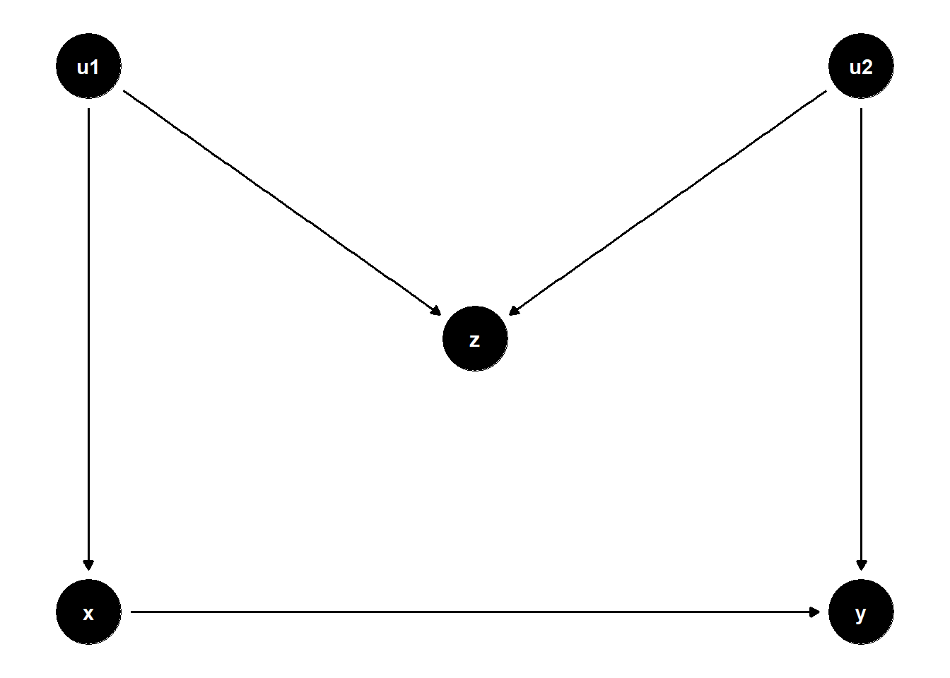
Figure 47.1: DAG illustrating M-bias: \(Z\) is a collider on the path \(X \leftarrow U_1 \to Z \leftarrow U_2 \to Y\), so conditioning on the pre-treatment \(Z\) opens a non-causal path between \(X\) and \(Y\).
In this structure, \(Z\) is a collider on the path \(X \leftarrow U_1 \rightarrow Z \leftarrow U_2 \rightarrow Y\). Controlling for \(Z\) opens this path, introducing a spurious association between \(X\) and \(Y\) even if none existed originally.
Even though \(Z\) is statistically correlated with both \(X\) and \(Y\), it is not a confounder, because it does not lie on a back-door path that needs to be blocked. Instead, adjusting for \(Z\) biases the estimate of the causal effect of \(X \to Y\).
Let’s illustrate this with a simulation:
set.seed(123)

n <- 1e4
u1 <- rnorm(n)
u2 <- rnorm(n)
z <- u1 + u2 + rnorm(n)
x <- u1 + rnorm(n)
causal_coef <- 2
y <- causal_coef * x - 4 * u2 + rnorm(n)

# Compare unadjusted and adjusted models
jtools::export_summs(
  lm(y ~ x),
  lm(y ~ x + z),
  model.names = c("Unadjusted", "Adjusted")
)| Unadjusted | Adjusted | |
|---|---|---|
| (Intercept) | 0.05 | 0.03 |
| (0.04) | (0.03) | |
| x | 2.01 *** | 2.80 *** |
| (0.03) | (0.03) | |
| z | -1.57 *** | |
| (0.02) | ||
| N | 10000 | 10000 |
| R2 | 0.32 | 0.57 |
| *** p < 0.001; ** p < 0.01; * p < 0.05. | ||
Notice how adjusting for \(Z\) changes the estimate of the effect of \(X\) on \(Y\), even though \(Z\) is not a true confounder. This is a textbook example of M-bias in practice.
47.1.1.1 Worse: M-bias with Direct Effect from Z to Y
A more difficult case arises when \(Z\) also has a direct effect on \(Y\). Consider the DAG in Figure 47.2:
# Clean workspace
rm(list = ls())

# DAG specification
model <- dagitty("dag{
  x -> y
  u1 -> x
  u1 -> z
  u2 -> z
  u2 -> y
  z -> y
}")

# Set latent variables
latents(model) <- c("u1", "u2")

# Coordinates for plotting
coordinates(model) <- list(
  x = c(x = 1, u1 = 1, z = 2, u2 = 3, y = 3),
  y = c(x = 1, u1 = 2, z = 1.5, u2 = 2, y = 1)
)

# Plot the DAG
ggdag(model) + theme_dag()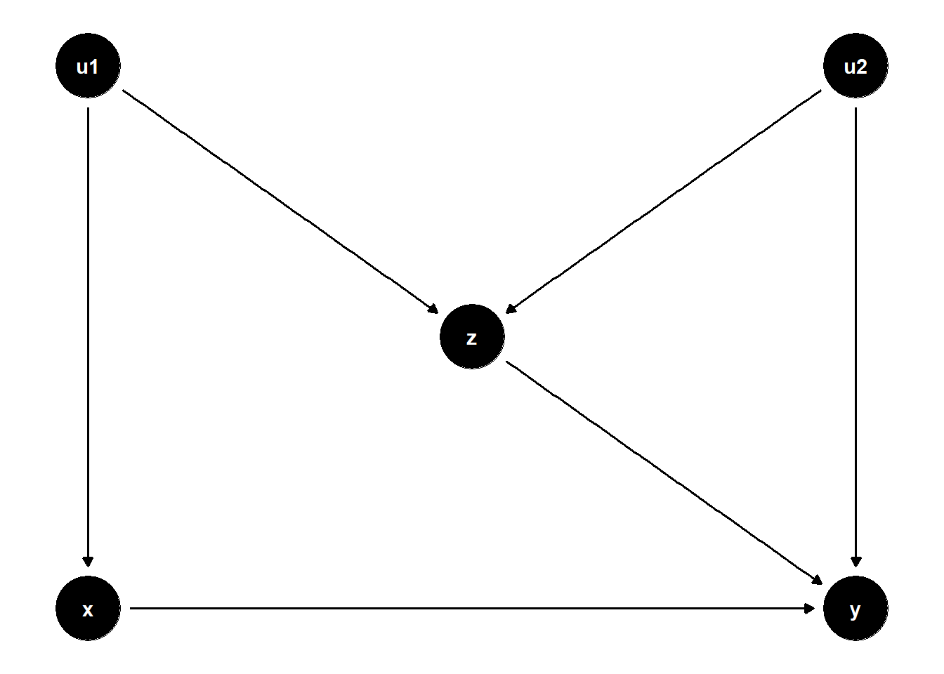
Figure 47.2: DAG illustrating the harder M-bias variant in which \(Z\) is both a collider and has a direct effect on \(Y\), so neither adjusting nor not adjusting for \(Z\) removes all bias.
This situation presents a dilemma:
Not controlling for \(Z\) leaves the back-door path \(X \leftarrow U_1 \to Z \to Y\) open, introducing confounding bias.
Controlling for \(Z\) opens the collider path \(X \leftarrow U_1 \to Z \leftarrow U_2 \to Y\), which also biases the estimate.
In short, no adjustment strategy can fully remove bias from the estimate of \(X \to Y\) using observed data alone.
What Can Be Done?
When facing such situations, we often turn to sensitivity analysis to assess how robust our causal conclusions are to unmeasured confounding. Specifically, recent advances (Cinelli et al. 2019; Cinelli and Hazlett 2020) allow us to quantify:
Plausible bounds on the strength of the direct effect \(Z \to Y\)
Sensitivity parameters reflecting the possible influence of the latent variables \(U_1\) and \(U_2\)
These tools help us understand how large the unmeasured biases would have to be in order to overturn our conclusions — a pragmatic approach when perfect control is impossible.
47.1.2 Bias Amplification
Bias amplification occurs when controlling for a variable that is not a confounder — in fact, controlling for it increases bias due to an unobserved confounder.
In the DAG in Figure 47.3, \(U\) is an unobserved common cause of both \(X\) and \(Y\). \(Z\) influences \(X\) but has no causal relationship with \(Y\). Including \(Z\) in the model does not block any back-door path but instead increases the bias from \(U\) by amplifying its association with \(X\).
# Clean workspace
rm(list = ls())

# DAG specification
model <- dagitty("dag{
  x -> y
  u -> x
  u -> y
  z -> x
}")

# Set latent variable
latents(model) <- c("u")

# Coordinates for plotting
coordinates(model) <- list(
  x = c(z = 1, x = 2, u = 3, y = 4),
  y = c(z = 1, x = 1, u = 2, y = 1)
)

# Plot the DAG
ggdag(model) + theme_dag()
Figure 47.3: DAG illustrating bias amplification: \(Z\) predicts \(X\) but is not a confounder, and adjusting for \(Z\) amplifies the omitted-variable bias from the unobserved common cause \(U\).
Even though \(Z\) is a strong predictor of \(X\), it is not a confounder, because it is not a common cause of \(X\) and \(Y\). Controlling for \(Z\) increases the portion of \(X\)’s variation explained by \(U\), thus amplifying bias in estimating the effect of \(X\) on \(Y\).
Simulation:
set.seed(123)
n <- 1e4
z <- rnorm(n)
u <- rnorm(n)
x <- 2*z + u + rnorm(n)
y <- x + 2*u + rnorm(n)

jtools::export_summs(
  lm(y ~ x),
  lm(y ~ x + z),
  model.names = c("Unadjusted", "Adjusted")
)| Unadjusted | Adjusted | |
|---|---|---|
| (Intercept) | -0.02 | -0.01 |
| (0.02) | (0.02) | |
| x | 1.32 *** | 1.99 *** |
| (0.01) | (0.01) | |
| z | -2.01 *** | |
| (0.03) | ||
| N | 10000 | 10000 |
| R2 | 0.71 | 0.80 |
| *** p < 0.001; ** p < 0.01; * p < 0.05. | ||
Observe that the adjusted model is more biased than the unadjusted one. This illustrates how controlling for a variable like \(Z\) can amplify omitted variable bias.
47.1.3 Overcontrol Bias
Overcontrol bias arises when we adjust for variables that lie on the causal path from treatment to outcome, or that serve as proxies for the outcome.
47.1.3.1 Mediator Control
Controlling for a mediator — a variable that lies on the causal path between treatment and outcome — removes part of the effect we are trying to estimate, as illustrated in Figure 47.4.
# Clean workspace
rm(list = ls())

# DAG: X → Z → Y
model <- dagitty("dag{
  x -> z
  z -> y
}")

coordinates(model) <- list(
  x = c(x = 1, z = 2, y = 3),
  y = c(x = 1, z = 1, y = 1)
)

ggdag(model) + theme_dag()
Figure 47.4: DAG illustrating mediator overcontrol: \(Z\) lies on the causal path \(X \to Z \to Y\), so conditioning on \(Z\) blocks part of the total effect of \(X\) on \(Y\).
If we want to estimate the total effect of \(X\) on \(Y\), controlling for \(Z\) (a mediator) leads to overcontrol bias.
set.seed(123)
n <- 1e4
x <- rnorm(n)
z <- x + rnorm(n)
y <- z + rnorm(n)

jtools::export_summs(
  lm(y ~ x),
  lm(y ~ x + z),
  model.names = c("Total Effect", "Controlled for Mediator")
)| Total Effect | Controlled for Mediator | |
|---|---|---|
| (Intercept) | -0.02 | -0.01 |
| (0.01) | (0.01) | |
| x | 1.03 *** | 0.02 |
| (0.01) | (0.01) | |
| z | 1.00 *** | |
| (0.01) | ||
| N | 10000 | 10000 |
| R2 | 0.34 | 0.67 |
| *** p < 0.001; ** p < 0.01; * p < 0.05. | ||
Here, \(Z\) will appear significant, but including it blocks the causal path from \(X\) to \(Y\). This is misleading when the goal is to estimate the total effect of \(X\).
47.1.3.2 Proxy for Mediator
In more complex scenarios, controlling for variables that proxy for mediators can introduce similar distortions, as in Figure 47.5.
# Clean workspace
rm(list = ls())

# DAG: X → M → Z, M → Y
model <- dagitty("dag{
  x -> m
  m -> z
  m -> y
}")

coordinates(model) <- list(
  x = c(x = 1, m = 2, z = 2, y = 3),
  y = c(x = 2, m = 2, z = 1, y = 2)
)

ggdag(model) + theme_dag()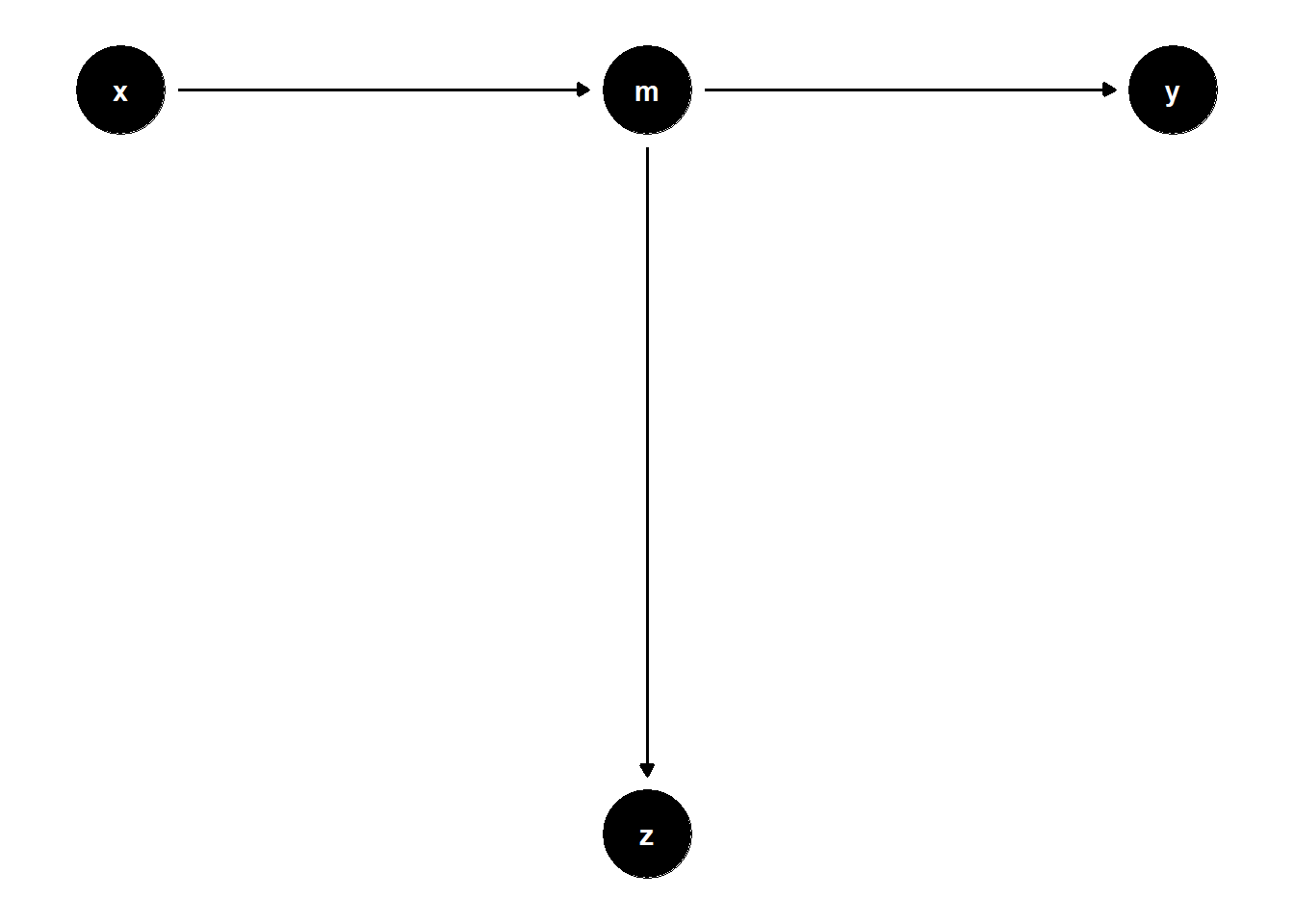
Figure 47.5: DAG illustrating proxy-for-mediator overcontrol: \(Z\) is a descendant of the mediator \(M\), so adjusting for \(Z\) partially blocks the indirect effect through \(M\).
set.seed(123)
n <- 1e4
x <- rnorm(n)
m <- x + rnorm(n)
z <- m + rnorm(n)
y <- m + rnorm(n)


jtools::export_summs(lm(y ~ x),
                     lm(y ~ x + z),
model.names = c("Total Effect", "Controlled for Proxy Z"))| Total Effect | Controlled for Proxy Z | |
|---|---|---|
| (Intercept) | -0.01 | -0.01 |
| (0.01) | (0.01) | |
| x | 0.99 *** | 0.49 *** |
| (0.01) | (0.02) | |
| z | 0.49 *** | |
| (0.01) | ||
| N | 10000 | 10000 |
| R2 | 0.33 | 0.49 |
| *** p < 0.001; ** p < 0.01; * p < 0.05. | ||
Even though \(Z\) is not on the path from \(X\) to \(Y\), controlling for it removes part of the causal variation coming through \(M\).
47.1.3.3 Overcontrol with Unobserved Confounding
When \(Z\) is influenced by both \(X\) and a latent confounder \(U\) that also affects \(Y\), controlling for \(Z\) again biases the estimate, as shown in Figure 47.6.
# Clean workspace
rm(list = ls())

# DAG: X → Z → Y; U → Z, U → Y
model <- dagitty("dag{
  x -> z
  z -> y
  u -> z
  u -> y
}")

latents(model) <- "u"

coordinates(model) <- list(
  x = c(x = 1, z = 2, u = 3, y = 4),
  y = c(x = 1, z = 1, u = 2, y = 1)
)

ggdag(model) + theme_dag()
Figure 47.6: DAG illustrating overcontrol with unobserved confounding: \(Z\) is a mediator that is also affected by a latent \(U\) which causes \(Y\), so adjusting for \(Z\) blocks the causal channel and opens a collider path through \(U\).
set.seed(1)
n <- 1e4
x <- rnorm(n)
u <- rnorm(n)
z <- x + u + rnorm(n)
y <- z + u + rnorm(n)

jtools::export_summs(
  lm(y ~ x),
  lm(y ~ x + z),
  model.names = c("Unadjusted", "Controlled for Z")
)| Unadjusted | Controlled for Z | |
|---|---|---|
| (Intercept) | -0.01 | -0.01 |
| (0.02) | (0.01) | |
| x | 1.01 *** | -0.47 *** |
| (0.02) | (0.01) | |
| z | 1.48 *** | |
| (0.01) | ||
| N | 10000 | 10000 |
| R2 | 0.15 | 0.78 |
| *** p < 0.001; ** p < 0.01; * p < 0.05. | ||
Although the total effect of \(X\) on \(Y\) is correctly captured in the unadjusted model, adjusting for \(Z\) introduces bias via the collider path \(X \to Z \leftarrow U \to Y\).
Insight: Controlling for \(Z\) inadvertently blocks the direct effect of \(X\) and opens a biasing path through \(U\). This makes the adjusted model unreliable for causal inference.
These examples highlight the importance of conceptual clarity and causal reasoning in model specification. Not all covariates should be controlled for — especially not those that are:
Mediators (on the causal path)
Proxies for mediators or outcomes
Colliders or descendants of colliders
In business contexts, this often arises when analysts include intermediate variables like sales leads, customer engagement scores, or operational metrics without understanding whether these mediate the effect of a treatment (e.g., ad spend) or confound it.
47.1.4 Selection Bias
Selection bias — also known as collider stratification bias — occurs when conditioning on a variable that is a collider (a common effect of two or more variables). This inadvertently opens non-causal paths, inducing spurious associations between variables that are otherwise independent or unconfounded.
Selection bias matters because it is rarely framed as a “control” decision in the first place. It often enters silently through sample restrictions, survey eligibility filters, or the way an outcome was operationalized, which means an analyst who never adds a single covariate to the regression can still be conditioning on a collider through the data they chose to observe. Recognizing the situation in practice usually starts with two questions: was a unit’s presence in the sample affected by the treatment or outcome, and does the dataset contain a variable that is a downstream consequence of both? When the answer is yes, the standard back-door adjustment intuition (see the Conditional Ignorability Assumption) breaks down even though every “confounder” appears to be controlled. Several of the cleanest fixes for this problem live outside the regression toolkit and instead exploit design-based identification, including Instrumental Variables and Quasi-Experimental approaches.
47.1.4.1 Classic Collider Bias
In the DAG in Figure 47.7, \(Z\) is a collider between \(X\) and a latent variable \(U\). Controlling for \(Z\) opens a back-door path from \(X\) to \(Y\) through \(U\), introducing bias.
rm(list = ls())

# DAG
model <- dagitty("dag{
  x -> y
  x -> z
  u -> z
  u -> y
}")
latents(model) <- "u"
coordinates(model) <- list(
  x = c(x = 1, z = 2, u = 2, y = 3),
  y = c(x = 3, z = 2, u = 4, y = 3)
)
ggdag(model) + theme_dag()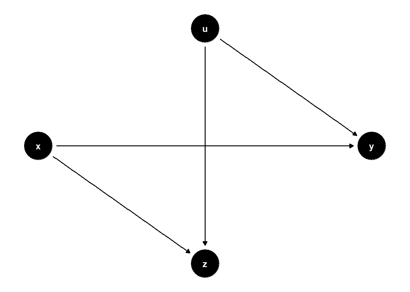
Figure 47.7: DAG illustrating classic collider bias: \(Z\) is a common effect of \(X\) and the latent \(U\), and conditioning on \(Z\) opens the non-causal path \(X \to Z \leftarrow U \to Y\).
Simulation:
set.seed(123)
n <- 1e4
x <- rnorm(n)
u <- rnorm(n)
z <- x + u + rnorm(n)
y <- x + 2*u + rnorm(n)

jtools::export_summs(
  lm(y ~ x),
  lm(y ~ x + z),
  model.names = c("Unadjusted", "Adjusted for Z (collider)")
)| Unadjusted | Adjusted for Z (collider) | |
|---|---|---|
| (Intercept) | -0.02 | -0.01 |
| (0.02) | (0.02) | |
| x | 0.99 *** | -0.02 |
| (0.02) | (0.02) | |
| z | 0.99 *** | |
| (0.01) | ||
| N | 10000 | 10000 |
| R2 | 0.17 | 0.49 |
| *** p < 0.001; ** p < 0.01; * p < 0.05. | ||
Controlling for \(Z\) opens the non-causal path \(X \to Z \leftarrow U \to Y\), resulting in biased estimates of the effect of \(X\) on \(Y\).
47.1.4.2 Collider Between Treatment and Outcome
In some cases, the collider is influenced directly by both the treatment and the outcome, as illustrated in Figure 47.8. This setting is also highly relevant in observational designs, particularly in retrospective or convenience sampling scenarios.
rm(list = ls())

# DAG: X → Z ← Y
model <- dagitty("dag{
  x -> y
  x -> z
  y -> z
}")
coordinates(model) <- list(
  x = c(x = 1, z = 2, y = 3),
  y = c(x = 2, z = 1, y = 2)
)
ggdag(model) + theme_dag()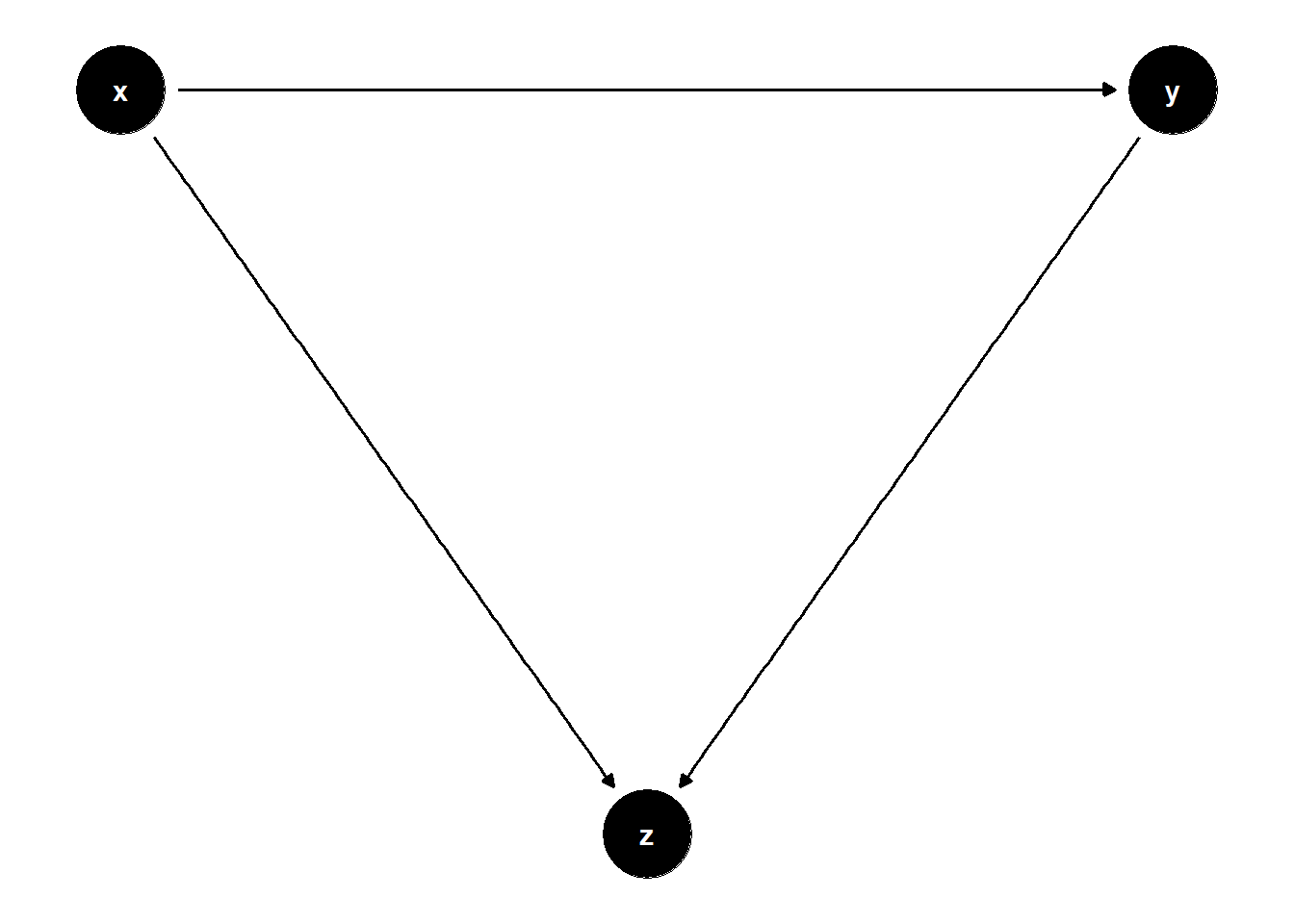
Figure 47.8: DAG illustrating a collider directly between treatment and outcome: \(Z\) is jointly caused by \(X\) and \(Y\), so conditioning on \(Z\) induces spurious dependence between \(X\) and \(Y\).
Simulation:
set.seed(123)
n <- 1e4
x <- rnorm(n)
y <- x + rnorm(n)
z <- x + y + rnorm(n)

jtools::export_summs(
  lm(y ~ x),
  lm(y ~ x + z),
  model.names = c("Unadjusted", "Adjusted for Collider Z")
)| Unadjusted | Adjusted for Collider Z | |
|---|---|---|
| (Intercept) | -0.01 | -0.00 |
| (0.01) | (0.01) | |
| x | 1.01 *** | -0.01 |
| (0.01) | (0.01) | |
| z | 0.50 *** | |
| (0.01) | ||
| N | 10000 | 10000 |
| R2 | 0.50 | 0.75 |
| *** p < 0.001; ** p < 0.01; * p < 0.05. | ||
Even though \(Z\) is associated with both \(X\) and \(Y\), it should not be controlled for, because doing so opens the collider path \(X \to Z \leftarrow Y\), generating spurious dependence.
47.1.5 Case-Control Bias
Case-control studies often condition on the outcome itself or on a descendant of the outcome, which can bias the estimated effect of the treatment on the outcome through several distinct mechanisms.
In the DAG in Figure 47.9, \(Z\) is a descendant of the outcome \(Y\) (not a descendant of a collider). Controlling for \(Z\) blocks part of the variation in \(Y\) that the treatment \(X\) induces and can attenuate or bias the estimated \(X \to Y\) effect.
rm(list = ls())

# DAG: X -> Y -> Z (Z is a descendant of the outcome Y)
model <- dagitty("dag{
  x -> y
  y -> z
}")
coordinates(model) <- list(
  x = c(x = 1, z = 2, y = 3),
  y = c(x = 2, z = 1, y = 2)
)
ggdag(model) + theme_dag()
Figure 47.9: DAG illustrating case-control bias: \(Z\) is a descendant of the outcome \(Y\) on the path \(X \to Y \to Z\), so conditioning on \(Z\) removes part of the treatment-induced variation in \(Y\).
Simulation:
set.seed(123)
n <- 1e4
x <- rnorm(n)
y <- x + rnorm(n)
z <- y + rnorm(n)

jtools::export_summs(
  lm(y ~ x),
  lm(y ~ x + z),
  model.names = c("Unadjusted", "Adjusted for Descendant Z")
)| Unadjusted | Adjusted for Descendant Z | |
|---|---|---|
| (Intercept) | -0.01 | -0.00 |
| (0.01) | (0.01) | |
| x | 1.01 *** | 0.49 *** |
| (0.01) | (0.01) | |
| z | 0.50 *** | |
| (0.01) | ||
| N | 10000 | 10000 |
| R2 | 0.50 | 0.75 |
| *** p < 0.001; ** p < 0.01; * p < 0.05. | ||
Note the subtlety: if \(X\) has a true causal effect on \(Y\), then controlling for \(Z\) (a descendant of \(Y\)) biases the estimate, because \(Z\) inherits the treatment-induced variation in \(Y\) and adjusting for it removes part of the channel \(X \to Y\) we are trying to measure. However, if \(X\) has no causal effect on \(Y\), then \(X\) remains d-separated from \(Y\) even when adjusting for \(Z\). In that special case, controlling for \(Z\) will not falsely suggest an effect.
Key Insight: Whether or not adjustment induces bias depends on the presence or absence of a true causal path. This highlights the importance of DAGs in clarifying assumptions and guiding valid statistical inference.
47.1.6 Summary
| Bias Type | Key Mistake | Path Opened | Consequence |
|---|---|---|---|
| M-Bias | Controlling for a collider | \(X \leftarrow U_1 \to Z \leftarrow U_2 \to Y\) | Spurious association |
| Bias Amplification | Controlling for a non-confounder | Amplifies unobserved confounding | Larger bias than before |
| Overcontrol Bias | Controlling for a mediator or proxy | Blocks part of causal effect | Underestimates total effect |
| Selection Bias | Conditioning on a collider or its descendant | \(X \to Z \leftarrow Y\) or similar | Induced non-causal correlation |
| Case-Control Bias | Conditioning on a descendant of the outcome | \(X \to Y \to Z\) | Attenuated \(X \to Y\) effect |
47.2 Good Controls
47.2.1 Omitted Variable Bias Correction
A variable \(Z\) is a good control when it blocks all back-door paths from the treatment \(X\) to the outcome \(Y\). This is the fundamental criterion from the back-door adjustment theorem in causal inference.
47.2.1.1 Simple Confounder
In the DAG in Figure 47.10, \(Z\) is a common cause of both \(X\) and \(Y\), i.e., a confounder.
rm(list = ls())

model <- dagitty("dag{
  x -> y
  z -> x
  z -> y
}")
coordinates(model) <- list(
  x = c(x = 1, z = 2, y = 3),
  y = c(x = 1, z = 2, y = 1)
)
ggdag(model) + theme_dag()
Figure 47.10: DAG illustrating a simple observed confounder: \(Z\) is a common cause of \(X\) and \(Y\), so adjusting for \(Z\) blocks the back-door path \(X \leftarrow Z \to Y\).
Controlling for \(Z\) removes the bias from the back-door path \(X \leftarrow Z \rightarrow Y\).
n <- 1e4
z <- rnorm(n)
causal_coef <- 2
beta2 <- 3
x <- z + rnorm(n)
y <- causal_coef * x + beta2 * z + rnorm(n)

jtools::export_summs(lm(y ~ x), lm(y ~ x + z))| Model 1 | Model 2 | |
|---|---|---|
| (Intercept) | -0.02 | 0.01 |
| (0.02) | (0.01) | |
| x | 3.49 *** | 2.00 *** |
| (0.02) | (0.01) | |
| z | 2.98 *** | |
| (0.01) | ||
| N | 10000 | 10000 |
| R2 | 0.82 | 0.97 |
| *** p < 0.001; ** p < 0.01; * p < 0.05. | ||
47.2.1.2 Confounding via a Latent Variable
In the structure in Figure 47.11, \(U\) is unobserved but causes both \(Z\) and \(Y\), and \(Z\) affects \(X\). Even though \(U\) is not observed, adjusting for \(Z\) helps block the back-door path from \(X\) to \(Y\) that goes through \(U\).
rm(list = ls())

model <- dagitty("dag{
  x -> y
  u -> z
  z -> x
  u -> y
}")
latents(model) <- "u"
coordinates(model) <- list(
  x = c(x = 1, z = 2, u = 3, y = 4),
  y = c(x = 1, z = 2, u = 3, y = 1)
)
ggdag(model) + theme_dag()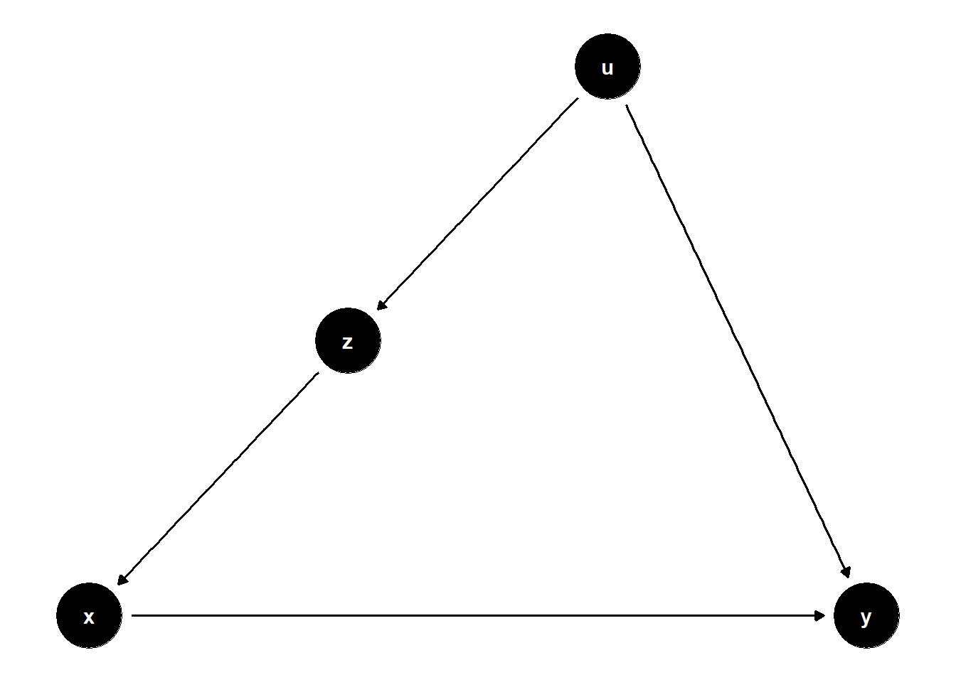
Figure 47.11: DAG illustrating an observed proxy for a latent confounder: \(U\) is unobserved and causes \(Z\) and \(Y\), while \(Z\) causes \(X\), so adjusting for \(Z\) blocks the back-door path \(X \leftarrow Z \leftarrow U \to Y\).
n <- 1e4
u <- rnorm(n)
z <- u + rnorm(n)
x <- z + rnorm(n)
y <- 2 * x + u + rnorm(n)

jtools::export_summs(lm(y ~ x), lm(y ~ x + z))| Model 1 | Model 2 | |
|---|---|---|
| (Intercept) | -0.02 | -0.01 |
| (0.01) | (0.01) | |
| x | 2.33 *** | 1.99 *** |
| (0.01) | (0.01) | |
| z | 0.51 *** | |
| (0.01) | ||
| N | 10000 | 10000 |
| R2 | 0.91 | 0.92 |
| *** p < 0.001; ** p < 0.01; * p < 0.05. | ||
Even though \(Z\) appears significant, its inclusion serves to reduce omitted variable bias rather than having a causal interpretation itself.
47.2.1.3 \(Z\) is caused by \(U\), but also causes \(Y\)
Figure 47.12 illustrates a subtle case where \(Z\) is on a non-causal path from \(X\) to \(Y\) and helps block bias through a shared cause \(U\).
rm(list = ls())

model <- dagitty("dag{
  x -> y
  u -> z
  u -> x
  z -> y
}")
latents(model) <- "u"
coordinates(model) <- list(
  x = c(x = 1, z = 3, u = 2, y = 4),
  y = c(x = 1, z = 2, u = 3, y = 1)
)
ggdag(model) + theme_dag()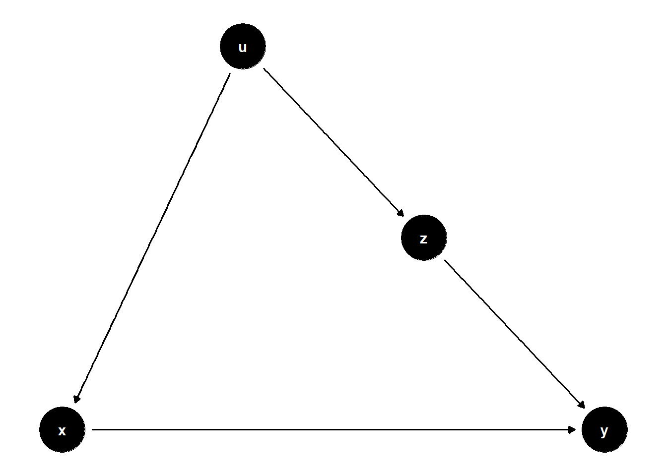
Figure 47.12: DAG illustrating a good control on a shared-cause path: \(U\) causes both \(Z\) and \(X\), \(Z\) causes \(Y\), and adjusting for \(Z\) blocks the back-door path \(X \leftarrow U \to Z \to Y\).
n <- 1e4
u <- rnorm(n)
z <- u + rnorm(n)
x <- u + rnorm(n)
y <- 2 * x + z + rnorm(n)

jtools::export_summs(lm(y ~ x), lm(y ~ x + z))| Model 1 | Model 2 | |
|---|---|---|
| (Intercept) | 0.02 | 0.01 |
| (0.02) | (0.01) | |
| x | 2.49 *** | 1.98 *** |
| (0.01) | (0.01) | |
| z | 1.02 *** | |
| (0.01) | ||
| N | 10000 | 10000 |
| R2 | 0.83 | 0.93 |
| *** p < 0.001; ** p < 0.01; * p < 0.05. | ||
Again, we cannot interpret the coefficient on \(Z\) causally, but including \(Z\) helps reduce omitted variable bias from the unobserved confounder \(U\).
47.2.1.4 Summary of Omitted Variable Correction
The three configurations above are summarized side-by-side in Figure 47.13.
# Model 1: Z is a confounder
model1 <- dagitty("dag{
  x -> y
  z -> x
  z -> y
}")
coordinates(model1) <-
    list(x = c(x = 1, z = 2, y = 3), y = c(x = 1, z = 2, y = 1))

# Model 2: Z is on path from U to X
model2 <- dagitty("dag{
  x -> y
  u -> z
  z -> x
  u -> y
}")
latents(model2) <- "u"
coordinates(model2) <-
    list(x = c(
        x = 1,
        z = 2,
        u = 3,
        y = 4
    ),
    y = c(
        x = 1,
        z = 2,
        u = 3,
        y = 1
    ))

# Model 3: Z influenced by U, affects Y
model3 <- dagitty("dag{
  x -> y
  u -> z
  u -> x
  z -> y
}")
latents(model3) <- "u"
coordinates(model3) <-
    list(x = c(
        x = 1,
        z = 3,
        u = 2,
        y = 4
    ),
    y = c(
        x = 1,
        z = 2,
        u = 3,
        y = 1
    ))

gridExtra::grid.arrange(
    ggdag(model1) + theme_dag(),
    ggdag(model2) + theme_dag(),
    ggdag(model3) + theme_dag(),
    nrow = 1
)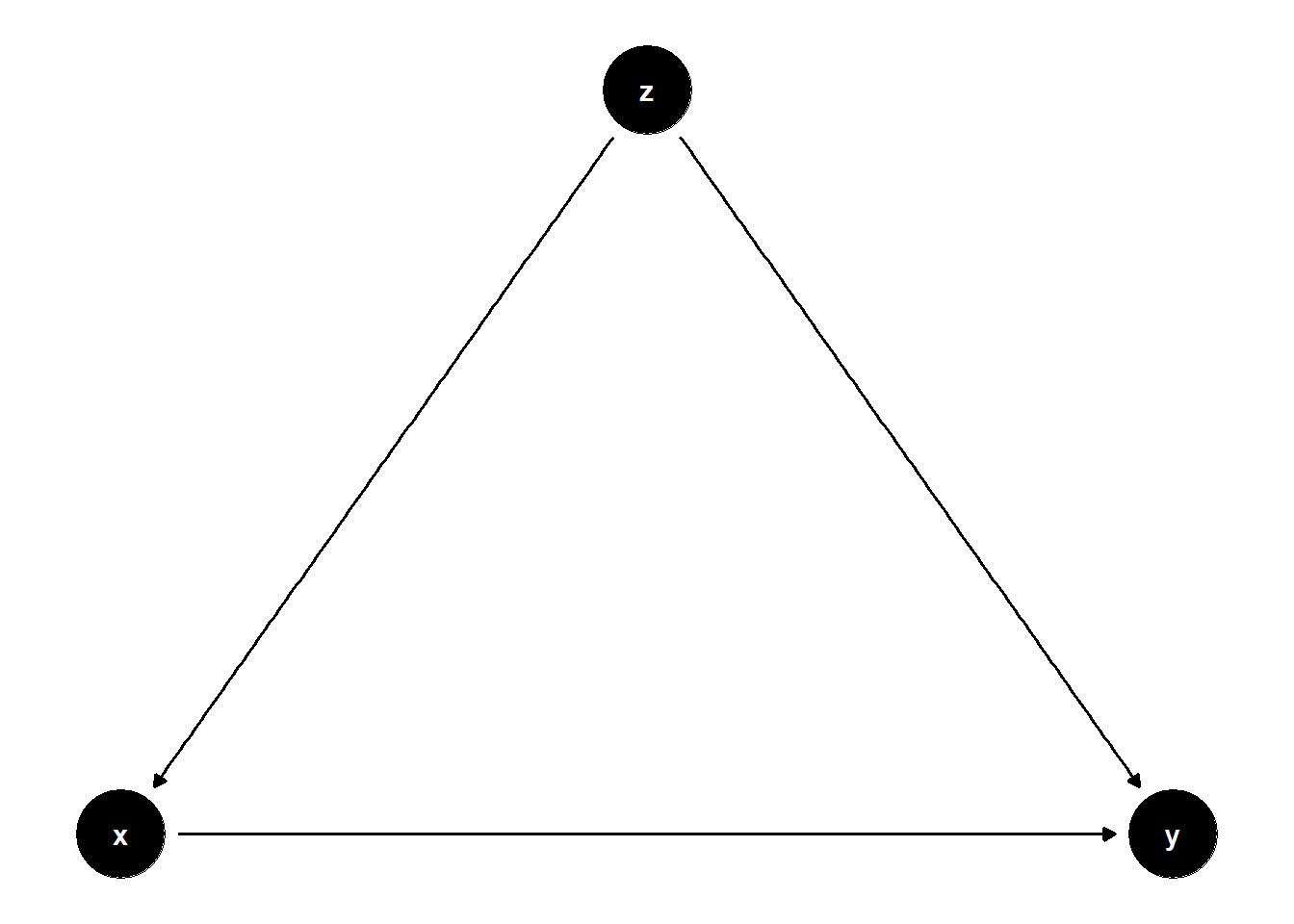
Figure 47.13: Summary panel of the three good-control DAGs for omitted-variable bias correction: a simple confounder, a latent confounder mediated through an observed \(Z\), and a shared cause \(U\) in which \(Z\) lies on the back-door path.
47.2.2 Omitted Variable Bias in Mediation Correction
When a variable \(Z\) is a confounder of both the treatment \(X\) and a mediator \(M\), controlling for \(Z\) helps isolate the indirect and direct effects more accurately.
47.2.2.1 Observed Confounder of Mediator and Treatment
Figure 47.14 shows the case in which \(Z\) is an observed common cause of both the treatment and the mediator.
rm(list = ls())

model <- dagitty("dag{
  x -> y
  z -> x
  x -> m
  z -> m
  m -> y
}")
coordinates(model) <-
    list(x = c(
        x = 1,
        z = 2,
        m = 3,
        y = 4
    ),
    y = c(
        x = 1,
        z = 2,
        m = 1,
        y = 1
    ))
ggdag(model) + theme_dag()
Figure 47.14: DAG illustrating mediation correction with an observed confounder: \(Z\) causes both the treatment \(X\) and the mediator \(M\), so adjusting for \(Z\) separates the indirect path \(X \to M \to Y\) from the back-door path through \(Z\).
n <- 1e4
z <- rnorm(n)
x <- z + rnorm(n)
m <- 2 * x + z + rnorm(n)
y <- m + rnorm(n)

jtools::export_summs(lm(y ~ x), lm(y ~ x + z))| Model 1 | Model 2 | |
|---|---|---|
| (Intercept) | -0.01 | 0.01 |
| (0.02) | (0.01) | |
| x | 2.50 *** | 1.99 *** |
| (0.01) | (0.01) | |
| z | 1.01 *** | |
| (0.02) | ||
| N | 10000 | 10000 |
| R2 | 0.84 | 0.87 |
| *** p < 0.001; ** p < 0.01; * p < 0.05. | ||
47.2.2.2 Latent Common Cause of Mediator and Treatment
Figure 47.15 extends the previous case to a latent confounder \(U\) that drives both the mediator and (indirectly) the treatment.
rm(list = ls())

model <- dagitty("dag{
  x -> y
  u -> z
  z -> x
  x -> m
  u -> m
  m -> y
}")
latents(model) <- "u"
coordinates(model) <-
    list(x = c(
        x = 1,
        z = 2,
        u = 3,
        m = 4,
        y = 5
    ),
    y = c(
        x = 1,
        z = 2,
        u = 3,
        m = 1,
        y = 1
    ))
ggdag(model) + theme_dag()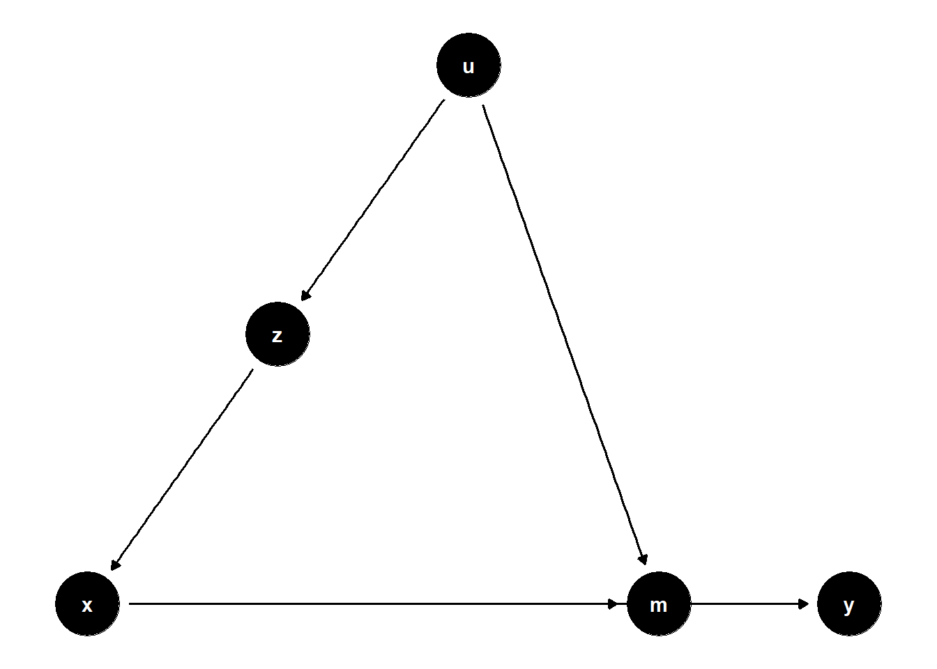
Figure 47.15: DAG illustrating mediation correction with a latent common cause: \(U\) is unobserved and causes both \(Z\) (which causes \(X\)) and the mediator \(M\), so adjusting for \(Z\) helps block the back-door path through \(U\).
n <- 1e4
u <- rnorm(n)
z <- u + rnorm(n)
x <- z + rnorm(n)
m <- 2 * x + u + rnorm(n)
y <- m + rnorm(n)

jtools::export_summs(lm(y ~ x), lm(y ~ x + z))| Model 1 | Model 2 | |
|---|---|---|
| (Intercept) | 0.01 | 0.01 |
| (0.02) | (0.02) | |
| x | 2.34 *** | 2.01 *** |
| (0.01) | (0.02) | |
| z | 0.50 *** | |
| (0.02) | ||
| N | 10000 | 10000 |
| R2 | 0.86 | 0.87 |
| *** p < 0.001; ** p < 0.01; * p < 0.05. | ||
47.2.2.3 Z Affects Mediator, U Affects Both X and Z
Figure 47.16 presents the variant in which \(Z\) acts on the mediator and a latent \(U\) jointly drives the treatment and \(Z\).
rm(list = ls())

model <- dagitty("dag{
  x -> y
  u -> z
  z -> m
  x -> m
  u -> x
  m -> y
}")
latents(model) <- "u"
coordinates(model) <-
    list(x = c(
        x = 1,
        z = 3,
        u = 2,
        m = 4,
        y = 5
    ),
    y = c(
        x = 1,
        z = 2,
        u = 3,
        m = 1,
        y = 1
    ))
ggdag(model) + theme_dag()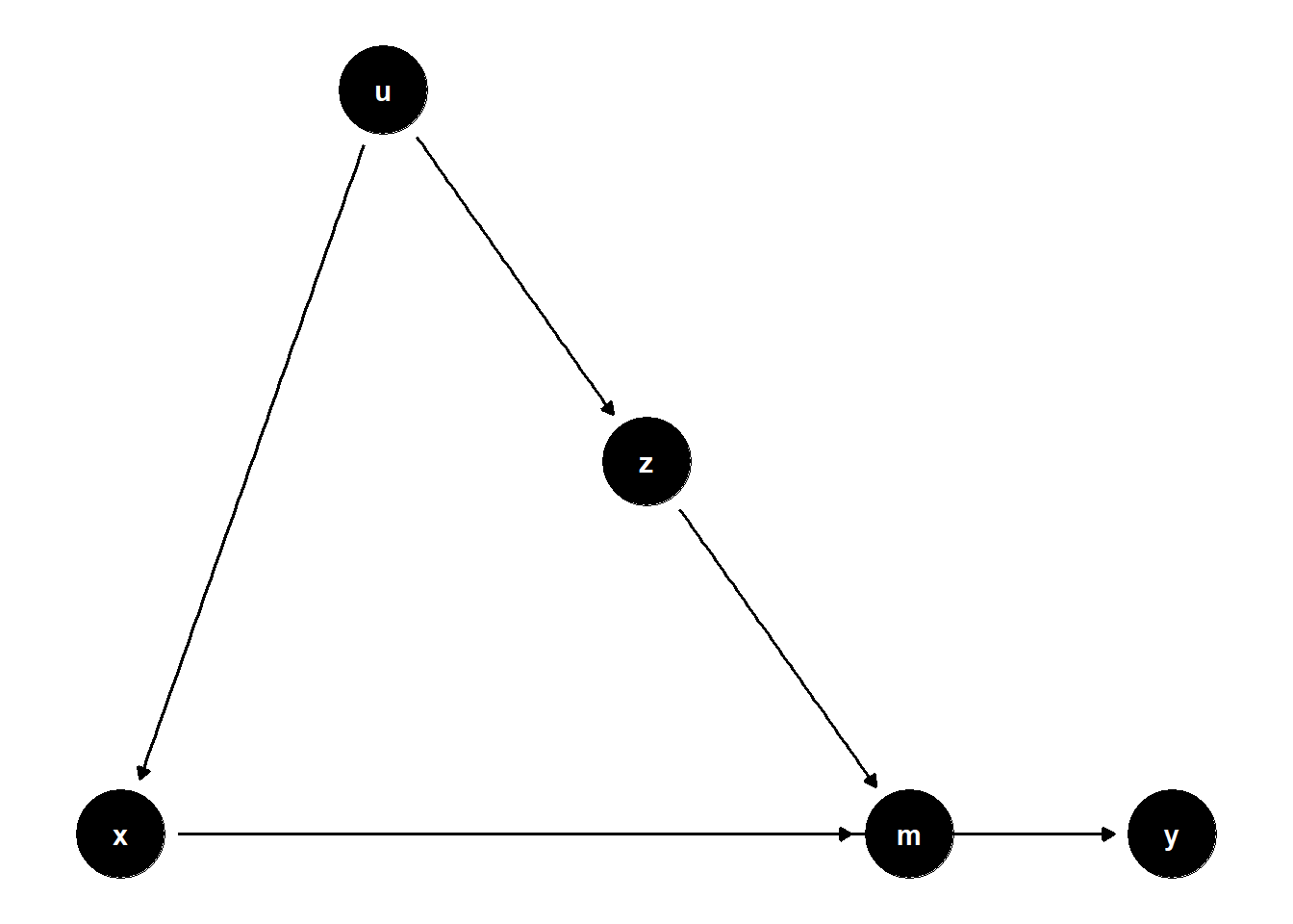
Figure 47.16: DAG illustrating mediation correction with \(Z\) as a parent of the mediator and a latent \(U\) that causes both \(X\) and \(Z\), so adjusting for \(Z\) blocks the back-door path through \(U\).
n <- 1e4
u <- rnorm(n)
z <- u + rnorm(n)
x <- u + rnorm(n)
m <- 2 * x + z + rnorm(n)
y <- m + rnorm(n)

jtools::export_summs(lm(y ~ x), lm(y ~ x + z))| Model 1 | Model 2 | |
|---|---|---|
| (Intercept) | 0.00 | 0.00 |
| (0.02) | (0.01) | |
| x | 2.49 *** | 1.99 *** |
| (0.01) | (0.01) | |
| z | 1.00 *** | |
| (0.01) | ||
| N | 10000 | 10000 |
| R2 | 0.78 | 0.87 |
| *** p < 0.001; ** p < 0.01; * p < 0.05. | ||
47.2.2.4 Summary of Mediation Correction
Figure 47.17 places the three mediation-correction DAGs side-by-side.
# Model 4
model4 <- dagitty("dag{
  x -> y
  z -> x
  x -> m
  z -> m
  m -> y
}")
coordinates(model4) <-
    list(x = c(
        x = 1,
        z = 2,
        m = 3,
        y = 4
    ),
    y = c(
        x = 1,
        z = 2,
        m = 1,
        y = 1
    ))

# Model 5
model5 <- dagitty("dag{
  x -> y
  u -> z
  z -> x
  x -> m
  u -> m
  m -> y
}")
latents(model5) <- "u"
coordinates(model5) <-
    list(x = c(
        x = 1,
        z = 2,
        u = 3,
        m = 4,
        y = 5
    ),
    y = c(
        x = 1,
        z = 2,
        u = 3,
        m = 1,
        y = 1
    ))

# Model 6
model6 <- dagitty("dag{
  x -> y
  u -> z
  z -> m
  x -> m
  u -> x
  m -> y
}")
latents(model6) <- "u"
coordinates(model6) <-
    list(x = c(
        x = 1,
        z = 3,
        u = 2,
        m = 4,
        y = 5
    ),
    y = c(
        x = 1,
        z = 2,
        u = 3,
        m = 1,
        y = 1
    ))

gridExtra::grid.arrange(
    ggdag(model4) + theme_dag(),
    ggdag(model5) + theme_dag(),
    ggdag(model6) + theme_dag(),
    nrow = 1
)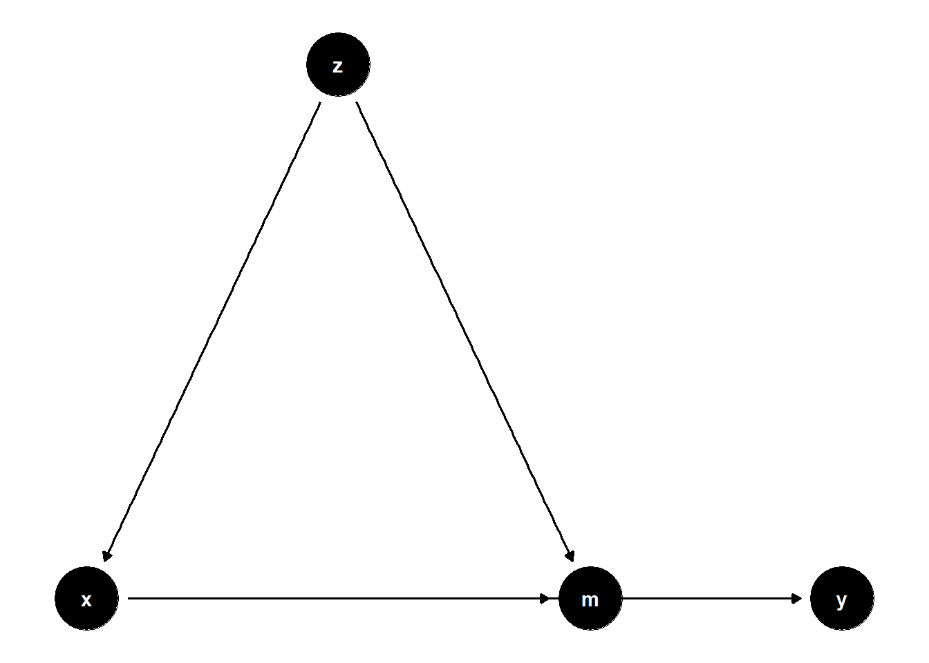
Figure 47.17: Summary panel of the three mediation-correction DAGs: an observed confounder of mediator and treatment, a latent common cause acting through an observed \(Z\), and the variant where \(Z\) acts on the mediator while \(U\) jointly causes \(X\) and \(Z\).
While \(Z\) may be statistically significant, this does not imply a causal effect unless \(Z\) is directly on the causal path from \(X\) to \(Y\). In many valid control scenarios, \(Z\) simply serves to isolate the causal effect of \(X\), not to be interpreted as a cause itself.
47.3 Neutral Controls
Not all covariates used in regression adjustment are necessary for identification. Neutral controls do not help with causal identification but may affect estimation precision. Including them:
- Does not introduce bias, because they do not lie on back-door or collider paths.
- May reduce standard errors, by explaining additional variation in the outcome.
47.3.1 Good Predictive Controls
When a variable is correlated with the outcome \(Y\), but not a cause of the treatment \(X\), controlling for it is optional for identification but may increase precision.
Good predictive controls matter because they are often the easiest free lunch in an applied analysis: they tighten standard errors without altering the point estimate or threatening identification. Recognizing them in practice means asking whether a candidate covariate has any plausible causal link back to the treatment. If the answer is no, and the variable independently moves the outcome, it acts like a baseline covariate in a randomized trial, soaking up residual variance in \(Y\) and shrinking the standard error on the treatment coefficient. The same logic underwrites the use of pre-treatment outcome levels in Difference-in-Differences and lagged covariates in Event Studies, where strong predictors of the outcome trajectory are routinely included for precision rather than identification.
47.3.1.1 \(Z\) predicts \(Y\), not \(X\)
Figure 47.18 shows the case in which \(Z\) has a direct effect on \(Y\) but no causal link to \(X\).
# Clean workspace
rm(list = ls())

model <- dagitty("dag{
  x -> y
  z -> y
}")
coordinates(model) <- list(
  x = c(x = 1, z = 2, y = 2),
  y = c(x = 1, z = 2, y = 1)
)
ggdag(model) + theme_dag()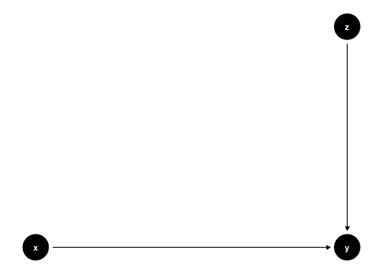
Figure 47.18: DAG illustrating a good predictive control: \(Z\) causes \(Y\) but is unrelated to \(X\), so adjusting for \(Z\) leaves the estimate of \(X \to Y\) unbiased while reducing residual variance.
n <- 1e4
z <- rnorm(n)
x <- rnorm(n)
y <- x + 2 * z + rnorm(n)

jtools::export_summs(
  lm(y ~ x),
  lm(y ~ x + z),
  model.names = c("Without Z", "With Predictive Z")
)| Without Z | With Predictive Z | |
|---|---|---|
| (Intercept) | -0.01 | -0.01 |
| (0.02) | (0.01) | |
| x | 1.01 *** | 1.01 *** |
| (0.02) | (0.01) | |
| z | 2.01 *** | |
| (0.01) | ||
| N | 10000 | 10000 |
| R2 | 0.17 | 0.83 |
| *** p < 0.001; ** p < 0.01; * p < 0.05. | ||
The coefficient on \(X\) remains unbiased in both models, but standard errors are smaller in the model with \(Z\).
47.3.1.2 \(Z\) predicts a mediator \(M\)
Figure 47.19 shows the variant in which \(Z\) predicts the mediator \(M\) rather than the outcome directly.
rm(list = ls())

model <- dagitty("dag{
  x -> y
  x -> m
  z -> m
  m -> y
}")
coordinates(model) <- list(
  x = c(x = 1, z = 2, m = 2, y = 3),
  y = c(x = 1, z = 2, m = 1, y = 1)
)
ggdag(model) + theme_dag()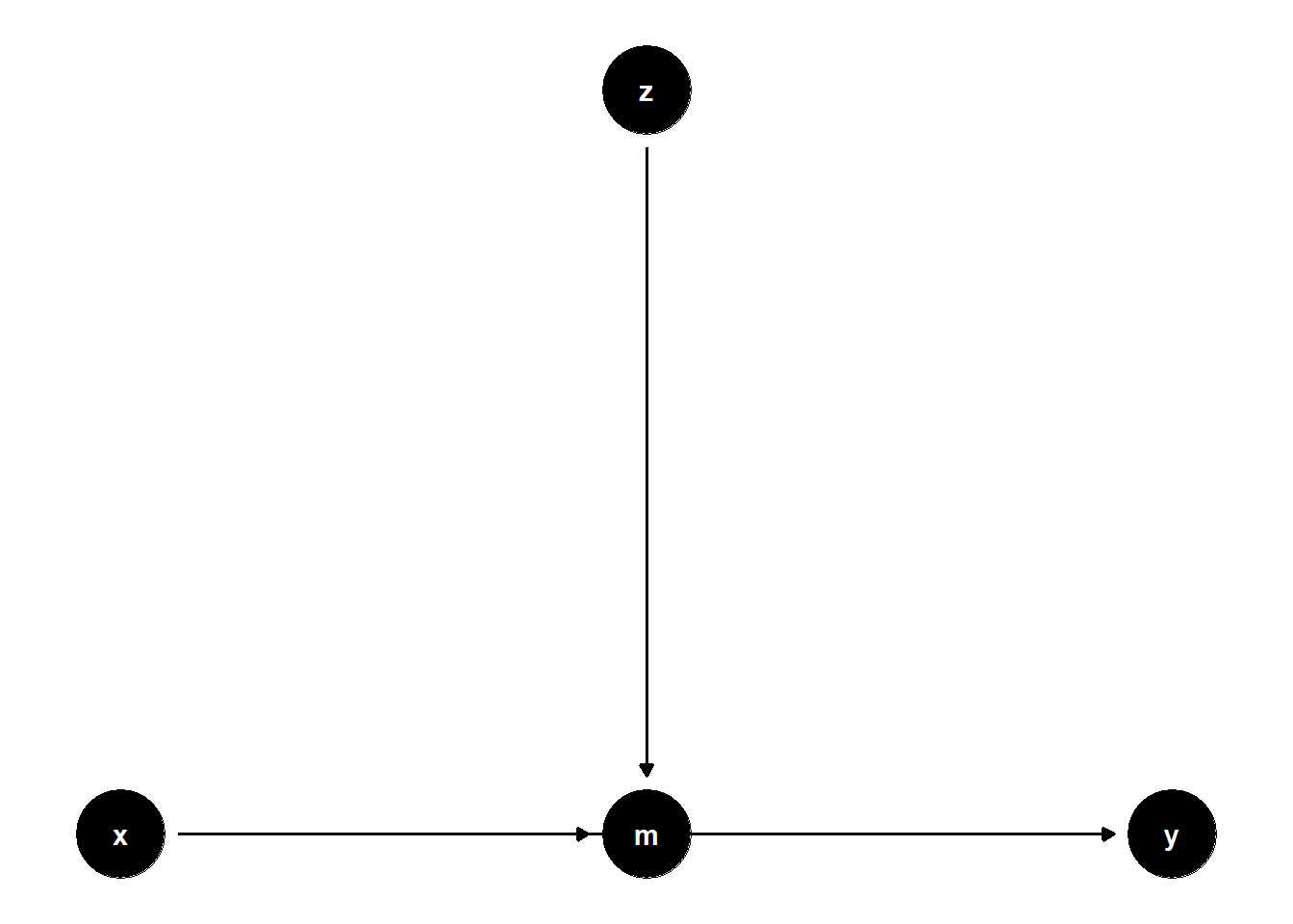
Figure 47.19: DAG illustrating a good predictive control acting on a mediator: \(Z\) causes the mediator \(M\) but is not on any causal path from \(X\) to \(Y\), so adjusting for \(Z\) reduces residual variance without bias.
n <- 1e4
z <- rnorm(n)
x <- rnorm(n)
m <- 2 * z + rnorm(n)
y <- x + 2 * m + rnorm(n)

jtools::export_summs(
  lm(y ~ x),
  lm(y ~ x + z),
  model.names = c("Without Z", "With Predictive Z")
)| Without Z | With Predictive Z | |
|---|---|---|
| (Intercept) | 0.02 | 0.02 |
| (0.05) | (0.02) | |
| x | 1.04 *** | 1.00 *** |
| (0.05) | (0.02) | |
| z | 3.98 *** | |
| (0.02) | ||
| N | 10000 | 10000 |
| R2 | 0.05 | 0.77 |
| *** p < 0.001; ** p < 0.01; * p < 0.05. | ||
Even though \(Z\) is not on any causal path from \(X\) to \(Y\), controlling for it may reduce residual variance in \(Y\), hence increasing precision.
47.3.2 Good Selection Bias
In more complex selection structures, adjusting for selection variables can improve identification, but only in the presence of additional post-selection information.
47.3.2.1 \(W\) is a collider; \(Z\) helps condition on selection
Figure 47.20 illustrates how an additional control \(Z\) can restore identification when conditioning on a downstream collider \(W\).
rm(list = ls())

model <- dagitty("dag{
  x -> y
  x -> z
  z -> w
  u -> w
  u -> y
}")
latents(model) <- "u"
coordinates(model) <- list(
  x = c(x = 1, z = 2, w = 3, u = 3, y = 5),
  y = c(x = 3, z = 2, w = 1, u = 4, y = 3)
)
ggdag(model) + theme_dag()
Figure 47.20: DAG illustrating good selection-bias adjustment: \(W\) is a collider with parents \(Z\) and \(U\), and adjusting for both \(W\) and \(Z\) blocks the otherwise-open path \(X \to Z \to W \leftarrow U \to Y\).
n <- 1e4
x <- rnorm(n)
u <- rnorm(n)
z <- x + rnorm(n)
w <- z + u + rnorm(n)
y <- x - 2 * u + rnorm(n)

jtools::export_summs(
  lm(y ~ x),
  lm(y ~ x + w),
  lm(y ~ x + z + w),
  model.names = c("Unadjusted", "Control W", "Control W + Z")
)| Unadjusted | Control W | Control W + Z | |
|---|---|---|---|
| (Intercept) | -0.00 | 0.00 | -0.02 |
| (0.02) | (0.02) | (0.02) | |
| x | 1.00 *** | 1.69 *** | 1.01 *** |
| (0.02) | (0.02) | (0.02) | |
| w | -0.67 *** | -1.00 *** | |
| (0.01) | (0.01) | ||
| z | 1.01 *** | ||
| (0.02) | |||
| N | 10000 | 10000 | 10000 |
| R2 | 0.18 | 0.40 | 0.51 |
| *** p < 0.001; ** p < 0.01; * p < 0.05. | |||
Unadjusted model is unbiased.
Controlling only for \(W\) is biased due to collider path \(X \to Z \to W \leftarrow U \to Y\).
Adding \(Z\) restores identification by blocking that path.
47.3.3 Bad Predictive Controls
Not all predictive variables are useful — some may reduce precision by soaking up degrees of freedom or increasing multicollinearity.
Bad predictive controls matter because they masquerade as good ones: they look statistically related to the treatment, they often improve in-sample fit, and a reviewer can reasonably ask why they were left out. Recognizing the situation in practice means flipping the question and asking what the variable predicts. A covariate that strongly predicts the treatment but adds nothing to explaining the outcome (beyond what the treatment already captures) competes with the treatment for variance and inflates the standard error on the causal coefficient. This is the same intuition that motivates the relevance condition in Instrumental Variables: a variable can be powerfully associated with \(X\) without being a useful adjustment, and the closer such a variable lies to a perfect predictor of \(X\), the more a regression that conditions on it begins to resemble a near-multicollinear specification.
47.3.3.1 \(Z\) predicts \(X\), not \(Y\)
Figure 47.21 illustrates the case in which \(Z\) predicts the treatment but does not affect the outcome.
rm(list = ls())

model <- dagitty("dag{
  x -> y
  z -> x
}")
coordinates(model) <- list(
  x = c(x = 1, z = 1, y = 2),
  y = c(x = 1, z = 2, y = 1)
)
ggdag(model) + theme_dag()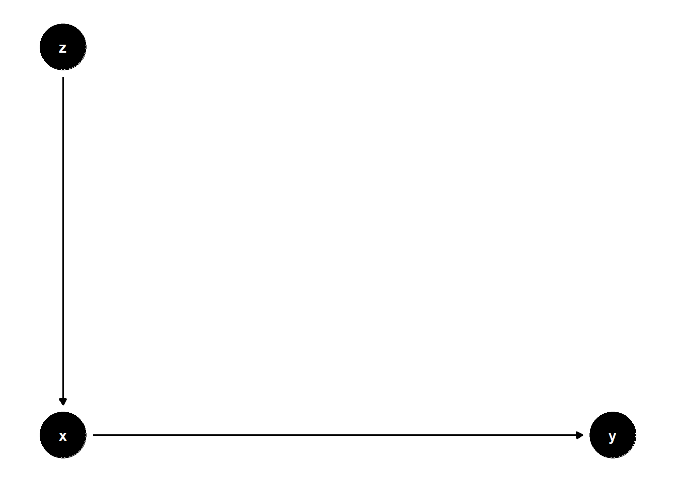
Figure 47.21: DAG illustrating a bad predictive control: \(Z\) causes \(X\) but has no effect on \(Y\), so conditioning on \(Z\) does not help identification and inflates the standard error on \(X\).
n <- 1e4
z <- rnorm(n)
x <- 2 * z + rnorm(n)
y <- x + rnorm(n)

jtools::export_summs(
  lm(y ~ x),
  lm(y ~ x + z),
  model.names = c("Without Z", "With Z (predicts X)")
)| Without Z | With Z (predicts X) | |
|---|---|---|
| (Intercept) | 0.01 | 0.01 |
| (0.01) | (0.01) | |
| x | 1.00 *** | 1.00 *** |
| (0.00) | (0.01) | |
| z | -0.00 | |
| (0.02) | ||
| N | 10000 | 10000 |
| R2 | 0.84 | 0.84 |
| *** p < 0.001; ** p < 0.01; * p < 0.05. | ||
\(Z\) adds no explanatory power for \(Y\), and thus increases SE for the estimate of \(X\)’s effect.
47.3.3.2 \(Z\) is a child of \(X\)
Figure 47.22 illustrates the post-treatment variant in which \(Z\) is a downstream effect of \(X\).
rm(list = ls())

model <- dagitty("dag{
  x -> y
  x -> z
}")
coordinates(model) <- list(
  x = c(x = 1, z = 1, y = 2),
  y = c(x = 1, z = 2, y = 1)
)
ggdag(model) + theme_dag()
Figure 47.22: DAG illustrating a post-treatment bad predictive control: \(Z\) is a child of \(X\) but does not affect \(Y\), so adjusting for \(Z\) inflates the standard error without contributing to identification.
n <- 1e4
x <- rnorm(n)
z <- 2 * x + rnorm(n)
y <- x + rnorm(n)

jtools::export_summs(
  lm(y ~ x),
  lm(y ~ x + z),
  model.names = c("Without Z", "With Child Z")
)| Without Z | With Child Z | |
|---|---|---|
| (Intercept) | 0.00 | 0.00 |
| (0.01) | (0.01) | |
| x | 1.02 *** | 1.06 *** |
| (0.01) | (0.02) | |
| z | -0.02 * | |
| (0.01) | ||
| N | 10000 | 10000 |
| R2 | 0.49 | 0.49 |
| *** p < 0.001; ** p < 0.01; * p < 0.05. | ||
Here, \(Z\) is a post-treatment variable. Though it does not bias the estimate of \(X\), it adds noise and increases the SE.
47.3.4 Bad Selection Bias
Controlling for some post-treatment variables can hurt precision without affecting bias, as in Figure 47.23.
rm(list = ls())

model <- dagitty("dag{
  x -> y
  x -> z
}")
coordinates(model) <- list(
  x = c(x = 1, z = 2, y = 2),
  y = c(x = 1, z = 2, y = 1)
)
ggdag(model) + theme_dag()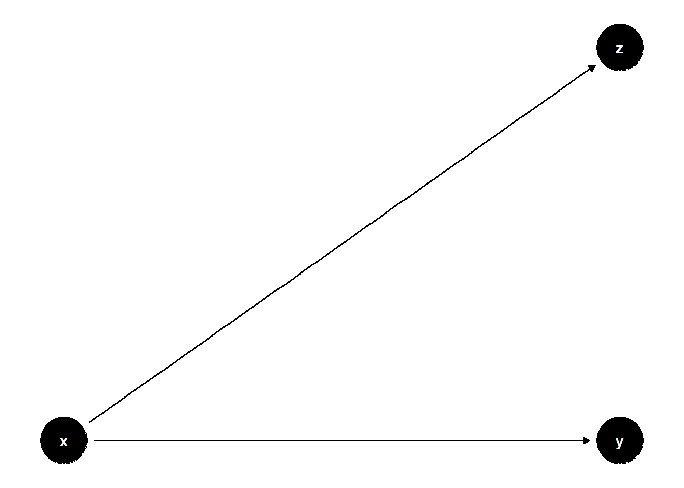
Figure 47.23: DAG illustrating a bad selection-bias control: \(Z\) is a post-treatment effect of \(X\) but is not on the causal path to \(Y\), so adjusting for \(Z\) does not introduce bias yet inflates the standard error.
n <- 1e4
x <- rnorm(n)
z <- 2 * x + rnorm(n)
y <- x + rnorm(n)

jtools::export_summs(
  lm(y ~ x),
  lm(y ~ x + z),
  model.names = c("Without Z", "With Post-treatment Z")
)| Without Z | With Post-treatment Z | |
|---|---|---|
| (Intercept) | -0.00 | -0.00 |
| (0.01) | (0.01) | |
| x | 1.00 *** | 0.99 *** |
| (0.01) | (0.02) | |
| z | 0.01 | |
| (0.01) | ||
| N | 10000 | 10000 |
| R2 | 0.50 | 0.50 |
| *** p < 0.001; ** p < 0.01; * p < 0.05. | ||
Although \(Z\) lies on a causal path from \(X\) to \(Z\) (and not from \(Z\) to \(Y\)), including \(Z\) adds redundant information and may inflate standard errors. In this case, it’s not a “bad control” in the M-bias sense, but still suboptimal.
47.3.5 Summary Table: Predictive vs. Causal Utility of Controls
| Control Type | Bias Impact | SE Impact | Causal Use? |
|---|---|---|---|
| Predictive of \(Y\), not \(X\) | None | Improves SE | Optional |
| Predictive of \(X\), not \(Y\) | None | Hurts SE | Avoid if possible |
| On causal path (\(X \to Z\)) | None (if not a mediator) | SE or undercontrol | Avoid unless estimating direct effect |
| Post-treatment collider | May induce bias | Hurts SE | Avoid |
| Aids blocking collider paths | May help | Mixed | Conditional |
47.4 Choosing Controls
Identifying which variables to control for is one of the most important — and difficult — steps in causal inference. The goal is to block all back-door paths between the treatment \(X\) and the outcome \(Y\), without introducing bias from colliders or mediators.
When done correctly, adjustment removes confounding bias. When done incorrectly, it can introduce bias, increase variance, or obscure the true causal relationship.
47.4.1 Step 1: Use a Causal Diagram (DAG)
Causal diagrams provide a graphical representation of assumptions about the data-generating process. With a DAG, we can:
- Identify all back-door paths from \(X\) to \(Y\)
- Determine which paths are blocked or opened by conditioning
- Use software to identify minimal sufficient adjustment sets
For example, using dagitty:
library(dagitty)

dag <- dagitty("dag {
  X -> Y
  Z -> X
  Z -> Y
  U -> X
  U -> Y
}")

adjustmentSets(dag, exposure = "X", outcome = "Y")
This will return the set(s) of covariates that must be controlled for to estimate the causal effect of \(X\) on \(Y\) under the back-door criterion.
47.4.2 Step 2: Use Algorithmic Tools
Several tools can automate the process of selecting appropriate controls given a DAG:
DAGitty provides an intuitive browser-based interface to:
Draw causal diagrams
Identify minimal sufficient adjustment sets
Simulate interventions (do-calculus)
Diagnose overcontrol or collider bias
It supports direct integration with R and allows reproducible workflows.
Fusion is a powerful tool for:
Computing identification formulas using do-calculus
Handling complex longitudinal data and selection bias
Formalizing queries for total, direct, and mediated effects
Fusion implements algorithms that go beyond standard adjustment and allow for nonparametric identification when latent confounders are present.
47.4.3 Step 3: Theoretical Principles
When the DAG is ambiguous or the analyst lacks software, a few theoretical principles do most of the work. They are essentially decision rules that translate the formal back-door criterion into questions an analyst can answer at the whiteboard. Each guideline below corresponds to a recurring pitfall already documented earlier in this chapter and to a chapter elsewhere in the book that handles the situation more carefully when adjustment alone is not enough.
Key guidelines include:
Do not control for mediators if estimating the total effect (see Mediation Analysis for direct/indirect-effect decomposition)
Control for pre-treatment confounders (common causes of treatment and outcome), which corresponds to Selection on Observables
Avoid colliders and their descendants, which trigger the Overcontrol Bias discussed earlier
Consider the use of Instrumental Variables when no suitable adjustment set exists, or related design-based fixes such as Regression Discontinuity, Difference-in-Differences, or Synthetic Control
47.4.4 Step 4: Consider Sensitivity Analysis
Even with well-reasoned DAGs, our control set may be imperfect, especially if some variables are unobserved or measured with error. In these cases, sensitivity analysis tools help quantify how robust our causal conclusions are.
The sensemakr package (Cinelli et al. 2019; Cinelli and Hazlett 2020) allows for:
Quantifying how strong unmeasured confounding would have to be to change conclusions
Reporting robustness values: the minimal strength of confounding needed to explain away the effect
Graphical summaries of confounding thresholds
This allows researchers to report assumptions transparently, even in the presence of unmeasured bias.
47.4.5 Step 5: Know When Not to Control
Remember, not every variable should be adjusted for. Table 47.1 summarises when to control and when to avoid.
| Variable Type | Control? | Why |
|---|---|---|
| Confounder (\(Z \to X\) and \(Z \to Y\)) | Yes | Blocks back-door path |
| Mediator (\(X \to Z \to Y\)) | No | Blocks part of the effect (unless estimating direct effect) |
| Collider (\(X \to Z \leftarrow Y\)) | No | Opens non-causal paths |
| Instrument (\(Z \to X\), \(Z \not\to Y\)) | No | Used differently, not for adjustment |
| Pre-treatment proxy for outcome | Caution | May amplify bias or introduce overcontrol |
| Predictor of outcome, not \(X\) | Optional | Improves precision, does not affect identification |
47.4.6 Summary: Control Selection Pipeline
Define your causal question clearly (total effect, direct effect, etc.)
Draw a DAG that reflects substantive knowledge
Use DAGitty/Fusion to identify minimal sufficient control sets
Double-check for bad controls (colliders, mediators)
If in doubt, conduct sensitivity analysis using
sensemakrReport assumptions transparently — causal conclusions are only as valid as the assumptions they rely on
The most important confounders are often unmeasured. But recognizing which ones should have been measured is already half the battle.