6 Non-Linear Regression

Moving beyond linearity, this chapter examines deterministic and stochastic non-linear models. We formalize inference under non-linear least squares, emphasize the distinction between intrinsic and extrinsic curvature, and explore identifiability issues.

Non-linear regression models differ fundamentally from linear regression models in that the derivatives of the mean function with respect to parameters depend on one or more of the parameters. This dependence adds complexity but also provides greater flexibility to model intricate relationships.

Linear Regression:

• Model Form Example: A typical linear regression model looks like \(y = \beta_0 + \beta_1 x\), where \(\beta_0\) and \(\beta_1\) are the parameters.

• Parameter Effect: The influence of each parameter on \(y\) is constant. For example, if \(\beta_1\) increases by 1, the change in \(y\) is always \(x\), regardless of the current value of \(\beta_1\).

• Derivatives: The partial derivatives of \(y\) with respect to each parameter (e.g., \(\frac{\partial y}{\partial \beta_1} = x\)) do not depend on the parameters \(\beta_0\) or \(\beta_1\) themselves. They only depend on the data \(x\). This makes the mathematics of finding the best-fit line straightforward.

• Straightforward estimation via closed-form solutions like Ordinary Least Squares.

Non-linear Regression:

• Model Form Example: Consider \(y = \alpha \cdot e^{\beta x}\). Here, \(\alpha\) and \(\beta\) are parameters, but the relationship is not a straight line.

• Parameter Effect: The effect of changing \(\alpha\) or \(\beta\) on \(y\) is not constant. For instance, if you change \(\beta\), the impact on \(y\) depends on both \(x\) and the current value of \(\beta\). This makes predictions and adjustments more complex.

• Derivatives: Taking the partial derivative with respect to \(\beta\) gives \(\frac{\partial y}{\partial \beta} = \alpha x e^{\beta x}\). Notice this derivative depends on \(\alpha\), \(\beta\), and \(x\). Unlike linear regression, the sensitivity of \(y\) to changes in \(\beta\) changes as \(\beta\) itself changes.

• Estimation requires iterative algorithms like the Gauss-Newton Algorithm, as closed-form solutions are not feasible.

Summary Table: Linear vs. Non-Linear Regression

Feature	Linear Regression	Non-Linear Regression
Relationship	Linear in parameters	Non-linear in parameters
Interpretability	High	Often challenging
Estimation	Closed-form solutions	Iterative algorithms
Computational Cost	Low	Higher

Key Features of Non-linear regression:

• Complex Functional Forms: Non-linear regression allows for relationships that are not straight lines or planes.
• Interpretability Challenges: Non-linear models can be difficult to interpret, especially if the functional forms are complex.
• Practical Use Cases:
  • Growth curves
  • High-order polynomials
  • Linear approximations (e.g., Taylor expansions)
  • Collections of locally linear models or basis functions (e.g., splines)

While these approaches can approximate data, they may suffer from interpretability issues or may not generalize well when data is sparse. Hence, intrinsically non-linear models are often preferred.

---

Intrinsically Non-Linear Models

The general form of an intrinsically non-linear regression model is:

\[ Y_i = f(\mathbf{x}_i; \mathbf{\theta}) + \epsilon_i \]

Where:

• \(f(\mathbf{x}_i; \mathbf{\theta})\): A non-linear function that relates \(E(Y_i)\) to the independent variables \(\mathbf{x}_i\).
• \(\mathbf{x}_i\): A \(k \times 1\) vector of independent variables (fixed).
• \(\mathbf{\theta}\): A \(p \times 1\) vector of parameters.
• \(\epsilon_i\): Independent and identically distributed random errors, often assumed to have a mean of 0 and a constant variance \(\sigma^2\). In some cases, \(\epsilon_i \sim \mathcal{N}(0, \sigma^2)\).

Example: Exponential Growth Model

A common non-linear model is the exponential growth function:

\[ y = \theta_1 e^{\theta_2 x} + \epsilon \]

Where:

• \(\theta_1\): Initial value.
• \(\theta_2\): Growth rate.
• \(x\): Independent variable (e.g., time).
• \(\epsilon\): Random error.

---

6.1 Inference

Since \(Y_i = f(\mathbf{x}_i, \theta) + \epsilon_i\), where \(\epsilon_i \sim \text{iid}(0, \sigma^2)\), we can estimate parameters (\(\hat{\theta}\)) by minimizing the sum of squared errors:

\[ \sum_{i=1}^{n} \big(Y_i - f(\mathbf{x}_i, \theta)\big)^2 \]

Let \(\hat{\theta}\) be the minimizer, the variance of residuals is estimated as:

\[ s^2 = \hat{\sigma}^2_{\epsilon} = \frac{\sum_{i=1}^{n} \big(Y_i - f(\mathbf{x}_i, \hat{\theta})\big)^2}{n - p} \]

where \(p\) is the number of parameters in \(\mathbf{\theta}\), and \(n\) is the number of observations.

---

Asymptotic Distribution of \(\hat{\theta}\)

Under regularity conditions (most notably that \(\epsilon_i \sim N(0, \sigma^2)\) or that \(n\) is sufficiently large for a central-limit-type argument), the parameter estimates \(\hat{\theta}\) have the following asymptotic normal distribution:

\[ \hat{\theta} \sim AN(\mathbf{\theta}, \sigma^2[\mathbf{F}(\theta)'\mathbf{F}(\theta)]^{-1}) \]

where

• \(AN\) stands for “asymptotic normality.”
• \(\mathbf{F}(\theta)\) is the \(n \times p\) Jacobian matrix of partial derivatives of \(f(\mathbf{x}_i, \theta)\) with respect to \(\mathbf{\theta}\), evaluated at \(\hat{\theta}\). Specifically,

\[ \mathbf{F}(\theta) = \begin{pmatrix} \frac{\partial f(\mathbf{x}_1, \boldsymbol{\theta})}{\partial \theta_1} & \cdots & \frac{\partial f(\mathbf{x}_1, \boldsymbol{\theta})}{\partial \theta_p} \\ \vdots & \ddots & \vdots \\ \frac{\partial f(\mathbf{x}_n, \boldsymbol{\theta})}{\partial \theta_1} & \cdots & \frac{\partial f(\mathbf{x}_n, \boldsymbol{\theta})}{\partial \theta_p} \end{pmatrix} \]

Asymptotic normality means that as the sample size \(n\) becomes large, the sampling distribution of \(\hat{\theta}\) approaches a normal distribution, which enables inference on the parameters.

6.1.1 Linear Functions of the Parameters

A “linear function of the parameters” refers to a quantity that can be written as \(\mathbf{a}'\boldsymbol{\theta}\), where \(\mathbf{a}\) is some (constant) contrast vector. Common examples include:

• A single parameter \(\theta_j\) (using a vector \(\mathbf{a}\) with 1 in the \(j\)-th position and 0 elsewhere).

• Differences, sums, or other contrasts, e.g. \(\theta_1 - \theta_2\).

Suppose we are interested in a linear combination of the parameters, such as \(\theta_1 - \theta_2\). Define the contrast vector \(\mathbf{a}\) as:

\[ \mathbf{a} = (0, 1, -1)' \]

We then consider inference for \(\mathbf{a'\theta}\) (\(\mathbf{a}\) can be \(p\)-dimensional vector). Using rules for the expectation and variance of a linear combination of a random vector \(\mathbf{Z}\):

\[ \begin{aligned} E(\mathbf{a'Z}) &= \mathbf{a'}E(\mathbf{Z}) \\ \text{Var}(\mathbf{a'Z}) &= \mathbf{a'} \text{Var}(\mathbf{Z}) \mathbf{a} \end{aligned} \]

We have

\[ \begin{aligned} E(\mathbf{a'\hat{\theta}}) &= \mathbf{a'}E(\hat{\theta}) \approx \mathbf{a}' \theta \\ \text{Var}(\mathbf{a'} \hat{\theta}) &= \mathbf{a'} \text{Var}(\hat{\theta}) \mathbf{a} \approx \sigma^2 \mathbf{a'[\mathbf{F}(\theta)'\mathbf{F}(\theta)]^{-1}a} \end{aligned} \]

Hence,

\[ \mathbf{a'\hat{\theta}} \sim AN\big(\mathbf{a'\theta}, \sigma^2 \mathbf{a'[\mathbf{F}(\theta)'\mathbf{F}(\theta)]^{-1}a}\big) \]

---

Confidence Intervals for Linear Contrasts

Since \(\mathbf{a'\hat{\theta}}\) is asymptotically independent of \(s^2\) (up to order \(O1/n\)), a two-sided \(100(1-\alpha)\%\) confidence interval for \(\mathbf{a'\theta}\) is given by:

\[ \mathbf{a'\theta} \pm t_{(1-\alpha/2, n-p)} s \sqrt{\mathbf{a'[\mathbf{F}(\hat{\theta})'\mathbf{F}(\hat{\theta})]^{-1}a}} \]

where

• \(t_{(1-\alpha/2, n-p)}\) is the critical value of the \(t\)-distribution with \(n - p\) degrees of freedom.
• \(s = \sqrt{\hat{\sigma^2}_\epsilon}\) is the estimated standard deviation of residuals.

Special Case: A Single Parameter \(\theta_j\)

If we focus on a single parameter \(\theta_j\), let \(\mathbf{a'} = (0, \dots, 1, \dots, 0)\) (with 1 at the \(j\)-th position). Then, the confidence interval for \(\theta_j\) becomes:

\[ \hat{\theta}_j \pm t_{(1-\alpha/2, n-p)} s \sqrt{\hat{c}^j} \]

where \(\hat{c}^j\) is the \(j\)-th diagonal element of \([\mathbf{F}(\hat{\theta})'\mathbf{F}(\hat{\theta})]^{-1}\).

---

6.1.2 Nonlinear Functions of Parameters

In many cases, we are interested in nonlinear functions of \(\boldsymbol{\theta}\). Let \(h(\boldsymbol{\theta})\) be such a function (e.g., a ratio of parameters, a difference of exponentials, etc.).

When \(h(\theta)\) is a nonlinear function of the parameters, we can use a Taylor series expansion about \(\theta\) to approximate \(h(\hat{\theta})\):

\[ h(\hat{\theta}) \approx h(\theta) + \mathbf{h}' [\hat{\theta} - \theta] \]

where

• \(\mathbf{h} = \left( \frac{\partial h}{\partial \theta_1}, \frac{\partial h}{\partial \theta_2}, \dots, \frac{\partial h}{\partial \theta_p} \right)'\) is the gradient vector of partial derivatives.

Key Approximations:

1. Expectation and Variance of \(\hat{\theta}\) (using the asymptotic normality of \(\hat{\theta}\): \[ \begin{aligned} E(\hat{\theta}) &\approx \theta, \\ \text{Var}(\hat{\theta}) &\approx \sigma^2 [\mathbf{F}(\theta)' \mathbf{F}(\theta)]^{-1}. \end{aligned} \]

2. Expectation and Variance of \(h(\hat{\theta})\) (properties of expectation and variance of (approximately) linear transformations): \[ \begin{aligned} E(h(\hat{\theta})) &\approx h(\theta), \\ \text{Var}(h(\hat{\theta})) &\approx \sigma^2 \mathbf{h}'[\mathbf{F}(\theta)' \mathbf{F}(\theta)]^{-1} \mathbf{h}. \end{aligned}\]

Combining these results, we find:

\[ h(\hat{\theta}) \sim AN(h(\theta), \sigma^2 \mathbf{h}' [\mathbf{F}(\theta)' \mathbf{F}(\theta)]^{-1} \mathbf{h}), \]

where \(AN\) represents asymptotic normality.

Confidence Interval for \(h(\theta)\):

An approximate \(100(1-\alpha)\%\) confidence interval for \(h(\theta)\) is:

\[ h(\hat{\theta}) \pm t_{(1-\alpha/2, n-p)} s \sqrt{\mathbf{h}'[\mathbf{F}(\theta)' \mathbf{F}(\theta)]^{-1} \mathbf{h}}, \]

where \(\mathbf{h}\) and \(\mathbf{F}(\theta)\) are evaluated at \(\hat{\theta}\).

---

To compute a prediction interval for a new observation \(Y_0\) at \(x = x_0\):

1. Model Definition: \[ Y_0 = f(x_0; \theta) + \epsilon_0, \quad \epsilon_0 \sim N(0, \sigma^2), \] with the predicted value: \[ \hat{Y}_0 = f(x_0, \hat{\theta}). \]

2. Approximation for \(\hat{Y}_0\): As \(n \to \infty\), \(\hat{\theta} \to \theta\), so we have: \[ f(x_0, \hat{\theta}) \approx f(x_0, \theta) + \mathbf{f}_0(\theta)' [\hat{\theta} - \theta], \] where: \[ \mathbf{f}_0(\theta) = \left( \frac{\partial f(x_0, \theta)}{\partial \theta_1}, \dots, \frac{\partial f(x_0, \theta)}{\partial \theta_p} \right)'. \]

3. Error Approximation: \[ \begin{aligned}Y_0 - \hat{Y}_0 &\approx Y_0 - f(x_0,\theta) - f_0(\theta)'[\hat{\theta}-\theta] \\&= \epsilon_0 - f_0(\theta)'[\hat{\theta}-\theta]\end{aligned} \]

4. Variance of \(Y_0 - \hat{Y}_0\): \[ \begin{aligned} \text{Var}(Y_0 - \hat{Y}_0) &\approx \text{Var}(\epsilon_0 - \mathbf{f}_0(\theta)' [\hat{\theta} - \theta]) \\ &= \sigma^2 + \sigma^2 \mathbf{f}_0(\theta)' [\mathbf{F}(\theta)' \mathbf{F}(\theta)]^{-1} \mathbf{f}_0(\theta) \\ &= \sigma^2 \big(1 + \mathbf{f}_0(\theta)' [\mathbf{F}(\theta)' \mathbf{F}(\theta)]^{-1} \mathbf{f}_0(\theta)\big). \end{aligned} \]

Hence, the prediction error \(Y_0 - \hat{Y}_0\) follows an asymptotic normal distribution:

\[ Y_0 - \hat{Y}_0 \sim AN\big(0, \sigma^2 \big(1 + \mathbf{f}_0(\theta)' [\mathbf{F}(\theta)' \mathbf{F}(\theta)]^{-1} \mathbf{f}_0(\theta)\big)\big). \]

A \(100(1-\alpha)\%\) prediction interval for \(Y_0\) is:

\[ \hat{Y}_0 \pm t_{(1-\alpha/2, n-p)} s \sqrt{1 + \mathbf{f}_0(\hat{\theta})' [\mathbf{F}(\hat{\theta})' \mathbf{F}(\hat{\theta})]^{-1} \mathbf{f}_0(\hat{\theta})}. \]

where we substitute \(\hat{\theta}\) into \(\mathbf{f}_0\) and \(\mathbf{F}\). Recall \(s\) is the estiamte of \(\sigma\).

---

Sometimes we want a confidence interval for \(E(Y_i)\) (i.e., the mean response at \(x_0\)), rather than a prediction interval for an individual future observation. In that case, the variance term for the random error \(\epsilon_0\) is not included. Hence, the formula is the same but without the “+1”:

\[ E(Y_0) \approx f(x_0; \theta), \]

and the confidence interval is:

\[ f(x_0, \hat{\theta}) \pm t_{(1-\alpha/2, n-p)} s \sqrt{\mathbf{f}_0(\hat{\theta})' [\mathbf{F}(\hat{\theta})' \mathbf{F}(\hat{\theta})]^{-1} \mathbf{f}_0(\hat{\theta})}. \]

Summary

• Linear Functions of the Parameters: A function \(f(x, \theta)\) is linear in \(\theta\) if it can be written in the form \[f(x, \theta) = \theta_1 g_1(x) + \theta_2 g_2(x) + \dots + \theta_p g_p(x)\] where \(g_j(x)\) do not depend on \(\theta\). In this case, the Jacobian \(\mathbf{F}(\theta)\) does not depend on \(\theta\) itself (only on \(x_i\)), and exact formulas often match what is familiar from linear regression.

• Nonlinear Functions of Parameters: If \(f(x, \theta)\) depends on \(\theta\) in a nonlinear way (e.g., \(\theta_1 e^{\theta_2 x}, \beta_1/\beta_2\) or more complicated expressions), \(\mathbf{F}(\theta)\) depends on \(\theta\). Estimation generally requires iterative numerical methods (e.g., Gauss–Newton, Levenberg–Marquardt), and the asymptotic results rely on evaluating partial derivatives at \(\hat{\theta}\). Nevertheless, the final inference formulas (e.g., confidence intervals, prediction intervals) have a similar form, thanks to the asymptotic normality arguments.

---

6.2 Non-linear Least Squares Estimation

The least squares (LS) estimate of \(\theta\), denoted as \(\hat{\theta}\), minimizes the residual sum of squares:

\[ S(\hat{\theta}) = SSE(\hat{\theta}) = \sum_{i=1}^{n} \{Y_i - f(\mathbf{x}_i; \hat{\theta})\}^2 \]

To solve this, we consider the partial derivatives of \(S(\theta)\) with respect to each \(\theta_j\) and set them to zero, leading to the normal equations:

\[ \frac{\partial S(\theta)}{\partial \theta_j} = -2 \sum_{i=1}^{n} \{Y_i - f(\mathbf{x}_i; \theta)\} \frac{\partial f(\mathbf{x}_i; \theta)}{\partial \theta_j} = 0 \]

However, these equations are inherently non-linear and, in most cases, cannot be solved analytically. As a result, various estimation techniques are employed to approximate solutions efficiently. These approaches include:

• Iterative Optimization – Methods that refine estimates through successive iterations to minimize error.
• [Derivative-Free] Methods – Techniques that do not rely on gradient information, useful for complex or non-smooth functions.
• Stochastic Heuristic – Algorithms that incorporate randomness, such as genetic algorithms or simulated annealing, to explore solution spaces.
• Linearization– Approximating non-linear models with linear ones to enable analytical or numerical solutions.
• Hybrid Approaches – Combining multiple methods to leverage their respective strengths for improved estimation.

Comparison of Optimization Methods for Nonlinear Estimation

Category	Method	Best For	Derivative?	Optimization	Comp. Cost
Iterative Optimization	Steepest Descent (Gradient Descent)	Simple problems, slow convergence	Yes	Local	Low
Iterative Optimization	Gauss-Newton Algorithm	Faster than GD, ignores exact second-order info	Yes	Local	Medium
Iterative Optimization	Levenberg-Marquardt Algorithm	Balances GN & GD, robust	Yes	Local	Medium
Iterative Optimization	Newton-Raphson Method	Quadratic convergence, needs Hessian	Yes	Local	High
Iterative Optimization	Quasi-Newton Method	Approximates Hessian for large problems	Yes	Local	Medium
Iterative Optimization	Trust-Region Reflective Algorithm	Handles constraints, robust	Yes	Local	High
Derivative-Free	Secant Method	Approximates derivative from function evaluations	No	Local	Medium
Derivative-Free	Nelder-Mead (Simplex)	No derivatives, heuristic	No	Local	Medium
Derivative-Free	Powell’s Method	Line search, no explicit gradient	No	Local	Medium
Derivative-Free	Grid Search	Exhaustive search (best in low dims)	No	Global	Very High
Derivative-Free	Hooke-Jeeves Pattern Search	Pattern-based, black-box optimization	No	Local	Medium
Derivative-Free	Bisection Method	Simple root/interval-based approach	No	Local	Low
Stochastic Heuristic	Simulated Annealing	Escapes local minima, non-smooth problems	No	Global	High
Stochastic Heuristic	Genetic Algorithm	Large search spaces, evolving parameters	No	Global	High
Stochastic Heuristic	Particle Swarm Optimization	Swarm-based, often fast global convergence	No	Global	Medium
Stochastic Heuristic	Evolutionary Strategies	High-dimensional, adaptive step-size	No	Global	High
Stochastic Heuristic	Differential Evolution Algorithm	Robust global optimizer, population-based	No	Global	High
Stochastic Heuristic	Ant Colony Optimization (ACO)	Discrete / combinatorial problems	No	Global	High
Linearization	Taylor Series Approximation	Local approximation of non-linearity	Yes	Local	Low
Linearization	Log-Linearization	Transforms non-linear equations	Yes	Local	Low
Hybrid	Adaptive Levenberg-Marquardt	Dynamically adjusts damping in LM	Yes	Local	Medium
Hybrid	Hybrid Genetic Algorithm & LM (GA-LM)	GA for coarse search, LM for fine-tuning	No	Hybrid	High
Hybrid	Neural Network-Based NLLS	Deep learning for complex non-linear least squares	No	Hybrid	Very High

---

6.2.1 Iterative Optimization

6.2.1.1 Gauss-Newton Algorithm

The Gauss-Newton Algorithm is an iterative optimization method used to estimate parameters in nonlinear least squares problems. It refines parameter estimates by approximating the Hessian matrix using first-order derivatives, making it computationally efficient for many practical applications (e.g., regression models in finance and marketing analytics). The objective is to minimize the Sum of Squared Errors (SSE):

\[ SSE(\theta) = \sum_{i=1}^{n} [Y_i - f_i(\theta)]^2, \]

where \(\mathbf{Y} = [Y_1, \dots, Y_n]'\) are the observed responses, and \(f_i(\theta)\) are the model-predicted values.

---

Iterative Refinement via Taylor Expansion

The Gauss-Newton algorithm iteratively refines an initial estimate \(\hat{\theta}^{(0)}\) using the Taylor series expansion of \(f(\mathbf{x}_i; \theta)\) about \(\hat{\theta}^{(0)}\). We start with the observation model:

\[ Y_i = f(\mathbf{x}_i; \theta) + \epsilon_i. \]

By expanding \(f(\mathbf{x}_i; \theta)\) around \(\hat{\theta}^{(0)}\) and ignoring higher-order terms (assuming the remainder is small), we get:

\[ \begin{aligned} Y_i &\approx f(\mathbf{x}_i; \hat{\theta}^{(0)}) + \sum_{j=1}^{p} \frac{\partial f(\mathbf{x}_i; \theta)}{\partial \theta_j} \bigg|_{\theta = \hat{\theta}^{(0)}} \left(\theta_j - \hat{\theta}_j^{(0)}\right) + \epsilon_i. \end{aligned} \]

In matrix form, let

\[ \mathbf{Y} = \begin{bmatrix} Y_1 \\ \vdots \\ Y_n \end{bmatrix}, \quad \mathbf{f}(\hat{\theta}^{(0)}) = \begin{bmatrix} f(\mathbf{x}_1, \hat{\theta}^{(0)}) \\ \vdots \\ f(\mathbf{x}_n, \hat{\theta}^{(0)}) \end{bmatrix}, \]

and define the Jacobian matrix of partial derivatives

\[ \mathbf{F}(\hat{\theta}^{(0)}) = \begin{bmatrix} \frac{\partial f(\mathbf{x}_1, \theta)}{\partial \theta_1} & \cdots & \frac{\partial f(\mathbf{x}_1, \theta)}{\partial \theta_p} \\ \vdots & \ddots & \vdots \\ \frac{\partial f(\mathbf{x}_n, \theta)}{\partial \theta_1} & \cdots & \frac{\partial f(\mathbf{x}_n, \theta)}{\partial \theta_p} \end{bmatrix}_{\theta = \hat{\theta}^{(0)}}. \]

Then,

\[ \mathbf{Y} \approx \mathbf{f}(\hat{\theta}^{(0)}) + \mathbf{F}(\hat{\theta}^{(0)})(\theta - \hat{\theta}^{(0)}) + \epsilon, \]

with \(\epsilon = [\epsilon_1, \dots, \epsilon_n]'\) assumed i.i.d. with mean \(0\) and variance \(\sigma^2\).

From this linear approximation,

\[ \mathbf{Y} - \mathbf{f}(\hat{\theta}^{(0)}) \approx \mathbf{F}(\hat{\theta}^{(0)})(\theta - \hat{\theta}^{(0)}). \]

Solving for \(\theta - \hat{\theta}^{(0)}\) in the least squares sense gives the Gauss increment \(\hat{\delta}^{(1)}\), so we can update:

\[ \hat{\theta}^{(1)} = \hat{\theta}^{(0)} + \hat{\delta}^{(1)}. \]

---

Step-by-Step Procedure

1. Initialize: Start with an initial estimate \(\hat{\theta}^{(0)}\) and set \(j = 0\).
2. Compute Taylor Expansion: Calculate \(\mathbf{f}(\hat{\theta}^{(j)})\) and \(\mathbf{F}(\hat{\theta}^{(j)})\).
3. Solve for Increment: Treating \(\mathbf{Y} - \mathbf{f}(\hat{\theta}^{(j)}) \approx \mathbf{F}(\hat{\theta}^{(j)}) (\theta - \hat{\theta}^{(j)})\) as a linear model, use Ordinary Least Squares to compute \(\hat{\delta}^{(j+1)}\).
4. Update Parameters: Set \(\hat{\theta}^{(j+1)} = \hat{\theta}^{(j)} + \hat{\delta}^{(j+1)}\).
5. Check for Convergence: If the convergence criteria are met (see below), stop; otherwise, return to Step 2.
6. Estimate Variance: After convergence, we assume \(\epsilon \sim (\mathbf{0}, \sigma^2 \mathbf{I})\). The variance \(\sigma^2\) can be estimated by

\[ \hat{\sigma}^2 = \frac{1}{n-p} \left(\mathbf{Y} - \mathbf{f}(\mathbf{x}; \hat{\theta})\right)' \left(\mathbf{Y} - \mathbf{f}(\mathbf{x}; \hat{\theta})\right). \]

---

Convergence Criteria

Common criteria for deciding when to stop iterating include:

1. Objective Function Change: \[ \frac{\left|SSE(\hat{\theta}^{(j+1)}) - SSE(\hat{\theta}^{(j)})\right|}{SSE(\hat{\theta}^{(j)})} < \gamma_1. \]
2. Parameter Change: \[ \left|\hat{\theta}^{(j+1)} - \hat{\theta}^{(j)}\right| < \gamma_2. \]
3. Residual Projection Criterion: The residuals satisfy convergence as defined in (Bates and Watts 1981).

---

Another way to see the update step is by viewing the necessary condition for a minimum: the gradient of \(SSE(\theta)\) with respect to \(\theta\) should be zero. For

\[ SSE(\theta) = \sum_{i=1}^{n} [Y_i - f_i(\theta)]^2, \]

the gradient is

\[ \frac{\partial SSE(\theta)}{\partial \theta} = 2\mathbf{F}(\theta)' \left[\mathbf{Y} - \mathbf{f}(\theta)\right]. \]

Using the Gauss-Newton update rule from iteration \(j\) to \(j+1\):

\[ \begin{aligned} \hat{\theta}^{(j+1)} &= \hat{\theta}^{(j)} + \hat{\delta}^{(j+1)} \\ &= \hat{\theta}^{(j)} + \left[\mathbf{F}(\hat{\theta}^{(j)})' \mathbf{F}(\hat{\theta}^{(j)})\right]^{-1} \mathbf{F}(\hat{\theta}^{(j)})' \left[\mathbf{Y} - \mathbf{f}(\hat{\theta}^{(j)})\right] \\ &= \hat{\theta}^{(j)} - \frac{1}{2} \left[\mathbf{F}(\hat{\theta}^{(j)})' \mathbf{F}(\hat{\theta}^{(j)})\right]^{-1} \frac{\partial SSE(\hat{\theta}^{(j)})}{\partial \theta}, \end{aligned} \]

where:

• \(\frac{\partial SSE(\hat{\theta}^{(j)})}{\partial \theta}\) is the gradient vector, pointing in the direction of steepest ascent of SSE.
• \(\left[\mathbf{F}(\hat{\theta}^{(j)})'\mathbf{F}(\hat{\theta}^{(j)})\right]^{-1}\) determines the step size, controlling how far to move in the direction of improvement.
• The factor \(-\tfrac{1}{2}\) ensures movement in the direction of steepest descent, helping to minimize the SSE.

The Gauss-Newton method works well when the nonlinear model can be approximated accurately by a first-order Taylor expansion near the solution. If the assumption of near-linearity in the residual function \(\mathbf{r}(\theta) = \mathbf{Y} - \mathbf{f}(\theta)\) is violated, convergence may be slow or fail altogether. In such cases, more robust methods like Levenberg-Marquardt Algorithm (which modifies Gauss-Newton with a damping parameter) are often preferred.

---

# Load necessary libraries
library(minpack.lm)  # Provides nonlinear least squares functions

# Define a nonlinear function (exponential model)
nonlinear_model <- function(theta, x) {
    # theta is a vector of parameters: theta[1] = A, theta[2] = B
    # x is the independent variable
    # The model is A * exp(B * x)
    theta[1] * exp(theta[2] * x)
}

# Define SSE function for clarity
sse <- function(theta, x, y) {
    # SSE = sum of squared errors between actual y and model predictions
    sum((y - nonlinear_model(theta, x)) ^ 2)
}

# Generate synthetic data
set.seed(123)                     # for reproducibility
x <- seq(0, 10, length.out = 100) # 100 points from 0 to 10
true_theta <- c(2, 0.3)           # true parameter values
y <- nonlinear_model(true_theta, x) + rnorm(length(x), sd = 0.5)

# Display the first few data points
head(data.frame(x, y))
#>           x        y
#> 1 0.0000000 1.719762
#> 2 0.1010101 1.946445
#> 3 0.2020202 2.904315
#> 4 0.3030303 2.225593
#> 5 0.4040404 2.322373
#> 6 0.5050505 3.184724

# Gauss-Newton optimization using nls.lm (Levenberg-Marquardt as extension).
# Initial guess for theta: c(1, 0.1)
fit <- nls.lm(
    par = c(1, 0.1),
    fn = function(theta)
        y - nonlinear_model(theta, x)
)

# Display estimated parameters
cat("Estimated parameters (A, B):\n")
#> Estimated parameters (A, B):
print(fit$par)
#> [1] 1.9934188 0.3008742

1. We defined the model “nonlinear_model(theta, x)” which returns Aexp(Bx).
2. We generated synthetic data using the “true_theta” values and added random noise.
3. We used nls.lm(...) from the minpack.lm package to fit the data:
   • par = c(1, 0.1) is our initial parameter guess.
   • fn = function(theta) y - nonlinear_model(theta, x) is the residual function, i.e., observed minus predicted.
4. The fit$par provides the estimated parameters after the algorithm converges.

# Visualize the data and the fitted model
plot(
  x,
  y,
  main = "Data and Fitted Curve (Gauss-Newton/Levenberg-Marquardt)",
  xlab = "x",
  ylab = "y",
  pch = 19,
  cex = 0.5
)
curve(
  nonlinear_model(fit$par, x),
  from = 0,
  to = 10,
  add = TRUE,
  col = "red",
  lwd = 2
)
legend(
  "topleft",
  legend = c("Data", "Fitted Curve"),
  pch = c(19, NA),
  lty = c(NA, 1),
  col = c("black", "red")
)

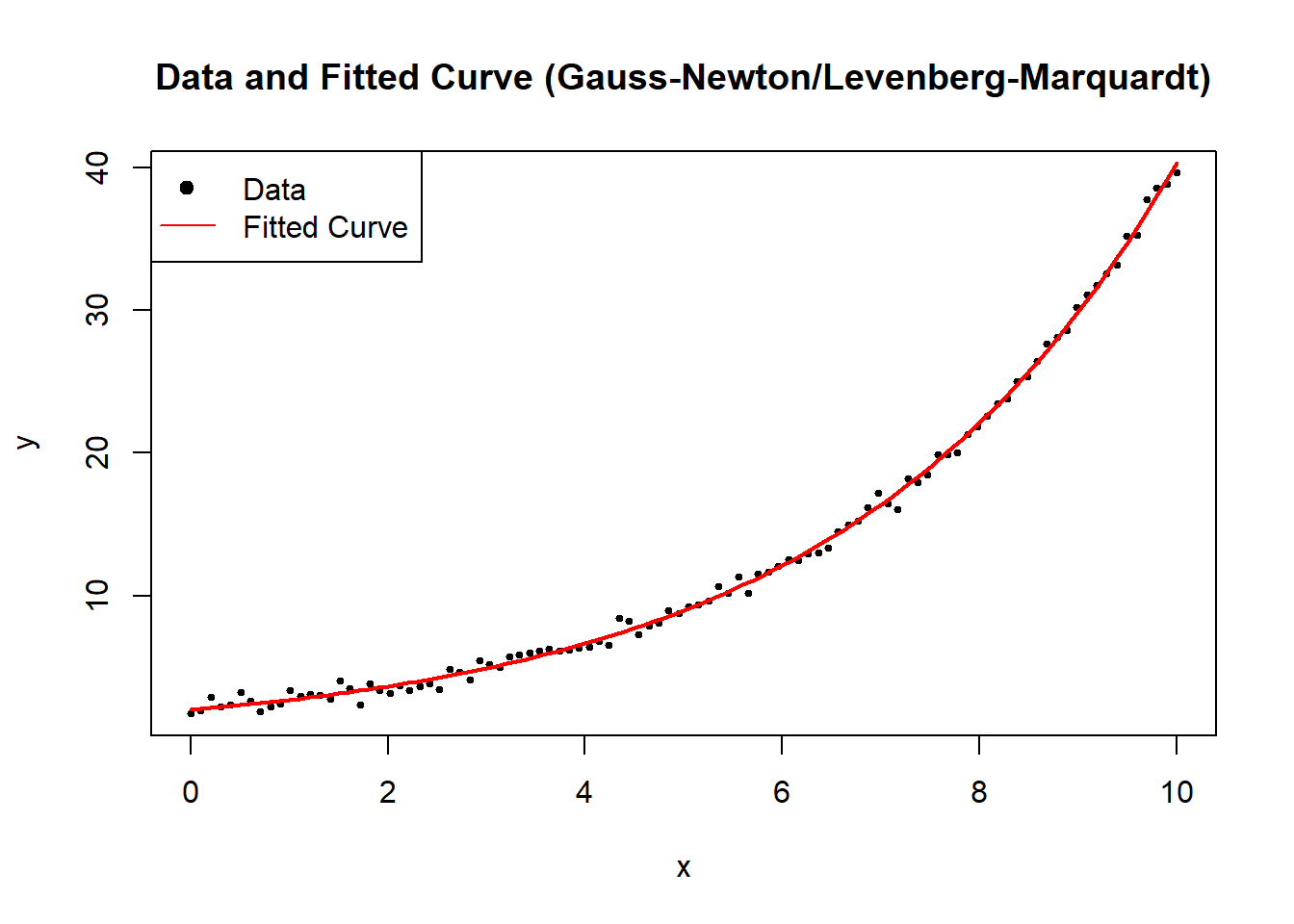
Figure 6.1: Data and Fitted Curve (Gauss–Newton/Levenberg–Marquardt)

6.2.1.2 Modified Gauss-Newton Algorithm

The Modified Gauss-Newton Algorithm introduces a learning rate \(\alpha_j\) to control step size and prevent overshooting the local minimum. The standard Gauss-Newton Algorithm assumes that the full step direction \(\hat{\delta}^{(j+1)}\) is optimal, but in practice, especially for highly nonlinear problems, it can overstep the minimum or cause numerical instability. The modification introduces a step size reduction, making it more robust.

We redefine the update step as:

\[ \hat{\theta}^{(j+1)} = \hat{\theta}^{(j)} + \alpha_j \hat{\delta}^{(j+1)}, \quad 0 < \alpha_j < 1, \]

where:

• \(\alpha_j\) is a learning rate, controlling how much of the step \(\hat{\delta}^{(j+1)}\) is taken.
• If \(\alpha_j = 1\), we recover the standard Gauss-Newton method.
• If \(\alpha_j\) is too small, convergence is slow; if too large, the algorithm may diverge.

This learning rate \(\alpha_j\) allows for adaptive step size adjustments, helping prevent excessive parameter jumps and ensuring that SSE decreases at each iteration.

---

A common approach to determine \(\alpha_j\) is step halving, ensuring that each iteration moves in a direction that reduces SSE. Instead of using a fixed \(\alpha_j\), we iteratively reduce the step size until SSE decreases:

\[ \hat{\theta}^{(j+1)} = \hat{\theta}^{(j)} + \frac{1}{2^k}\hat{\delta}^{(j+1)}, \]

where:

• \(k\) is the smallest non-negative integer such that

\[ SSE(\hat{\theta}^{(j)} + \frac{1}{2^k} \hat{\delta}^{(j+1)}) < SSE(\hat{\theta}^{(j)}). \]

This means we start with the full step \(\hat{\delta}^{(j+1)}\), then try \(\hat{\delta}^{(j+1)}/2\), then \(\hat{\delta}^{(j+1)}/4\), and so on, until SSE is reduced.

Algorithm for Step Halving:

1. Compute the Gauss-Newton step \(\hat{\delta}^{(j+1)}\).
2. Set an initial \(\alpha_j = 1\).
3. If the updated parameters \(\hat{\theta}^{(j)} + \alpha_j \hat{\delta}^{(j+1)}\) increase SSE, divide \(\alpha_j\) by 2.
4. Repeat until SSE decreases.

This ensures monotonic SSE reduction, preventing divergence due to an overly aggressive step.

---

Generalized Form of the Modified Algorithm

A more general form of the update rule, incorporating step size control and a matrix \(\mathbf{A}_j\), is:

\[ \hat{\theta}^{(j+1)} = \hat{\theta}^{(j)} - \alpha_j \mathbf{A}_j \frac{\partial Q(\hat{\theta}^{(j)})}{\partial \theta}, \]

where:

• \(\mathbf{A}_j\) is a positive definite matrix that preconditions the update direction.
• \(\alpha_j\) is the learning rate.
• \(\frac{\partial Q(\hat{\theta}^{(j)})}{\partial \theta}\) is the gradient of the objective function \(Q(\theta)\), typically SSE in nonlinear regression.

---

Connection to the Modified Gauss-Newton Algorithm

The Modified Gauss-Newton Algorithm fits this framework:

\[ \hat{\theta}^{(j+1)} = \hat{\theta}^{(j)} - \alpha_j [\mathbf{F}(\hat{\theta}^{(j)})' \mathbf{F}(\hat{\theta}^{(j)})]^{-1} \frac{\partial SSE(\hat{\theta}^{(j)})}{\partial \theta}. \]

Here, we recognize:

• Objective function: \(Q = SSE\).
• Preconditioner matrix: \([\mathbf{F}(\hat{\theta}^{(j)})' \mathbf{F}(\hat{\theta}^{(j)})]^{-1} = \mathbf{A}\).

Thus, the standard Gauss-Newton method can be interpreted as a special case of this broader optimization framework, with a preconditioned gradient descent approach.

---

# Load required library
library(minpack.lm)

# Define a nonlinear function (exponential model)
nonlinear_model <- function(theta, x) {
  theta[1] * exp(theta[2] * x)
}

# Define the Sum of Squared Errors function
sse <- function(theta, x, y) {
  sum((y - nonlinear_model(theta, x)) ^ 2)
}

# Generate synthetic data
set.seed(123)
x <- seq(0, 10, length.out = 100)
true_theta <- c(2, 0.3)
y <- nonlinear_model(true_theta, x) + rnorm(length(x), sd = 0.5)

# Gauss-Newton with Step Halving
gauss_newton_modified <-
  function(theta_init,
           x,
           y,
           tol = 1e-6,
           max_iter = 100) {
    theta <- theta_init
    for (j in 1:max_iter) {
      # Compute Jacobian matrix numerically
      epsilon <- 1e-6
      F_matrix <-
        matrix(0, nrow = length(y), ncol = length(theta))
      for (p in 1:length(theta)) {
        theta_perturb <- theta
        theta_perturb[p] <- theta[p] + epsilon
        F_matrix[, p] <-
          (nonlinear_model(theta_perturb, x)-nonlinear_model(theta, x))/epsilon
      }
      
      # Compute residuals
      residuals <- y - nonlinear_model(theta, x)
      
      # Compute Gauss-Newton step
      delta <-
        solve(t(F_matrix) %*% F_matrix) %*% t(F_matrix) %*% residuals
      
      # Step Halving Implementation
      alpha <- 1
      k <- 0
      while (sse(theta + alpha * delta, x, y) >= sse(theta, x, y) &&
             k < 10) {
        alpha <- alpha / 2
        k <- k + 1
      }
      
      # Update theta
      theta_new <- theta + alpha * delta
      
      # Check for convergence
      if (sum(abs(theta_new - theta)) < tol) {
        break
      }
      
      theta <- theta_new
    }
    return(theta)
  }

# Run Modified Gauss-Newton Algorithm
theta_init <- c(1, 0.1)  # Initial parameter guess
estimated_theta <- gauss_newton_modified(theta_init, x, y)

# Display estimated parameters
cat("Estimated parameters (A, B) with Modified Gauss-Newton:\n")
#> Estimated parameters (A, B) with Modified Gauss-Newton:
print(estimated_theta)
#>           [,1]
#> [1,] 1.9934188
#> [2,] 0.3008742

# Plot data and fitted curve
plot(
  x,
  y,
  main = "Modified Gauss-Newton: Data & Fitted Curve",
  pch = 19,
  cex = 0.5,
  xlab = "x",
  ylab = "y"
)
curve(
  nonlinear_model(estimated_theta, x),
  from = 0,
  to = 10,
  add = TRUE,
  col = "red",
  lwd = 2
)
legend(
  "topleft",
  legend = c("Data", "Fitted Curve"),
  pch = c(19, NA),
  lty = c(NA, 1),
  col = c("black", "red")
)

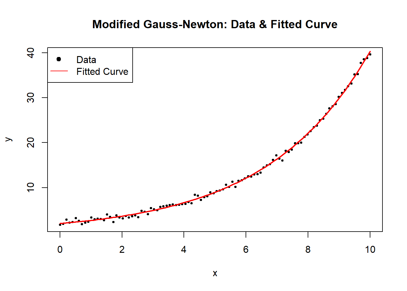
Figure 6.2: Modified Gauss–Newton

6.2.1.3 Steepest Descent (Gradient Descent)

The Steepest Descent Method, commonly known as Gradient Descent, is a fundamental iterative optimization technique used for finding parameter estimates that minimize an objective function \(\mathbf{Q}(\theta)\). It is a special case of the Modified Gauss-Newton Algorithm, where the preconditioning matrix \(\mathbf{A}_j\) is replaced by the identity matrix.

The update rule is given by:

\[ \hat{\theta}^{(j+1)} = \hat{\theta}^{(j)} - \alpha_j \mathbf{I}_{p \times p}\frac{\partial \mathbf{Q}(\hat{\theta}^{(j)})}{\partial \theta}, \]

where:

• \(\alpha_j\) is the learning rate, determining the step size.
• \(\mathbf{I}_{p \times p}\) is the identity matrix, meaning updates occur in the direction of the negative gradient.
• \(\frac{\partial \mathbf{Q}(\hat{\theta}^{(j)})}{\partial \theta}\) is the gradient vector, which provides the direction of steepest ascent; its negation ensures movement toward the minimum.

Characteristics of Steepest Descent

• Slow to converge: The algorithm moves in the direction of the gradient but does not take into account curvature, which may result in slow convergence, especially in ill-conditioned problems.
• Moves rapidly initially: The method can exhibit fast initial progress, but as it approaches the minimum, step sizes become small, leading to slow convergence.
• Useful for initialization: Due to its simplicity and ease of implementation, it is often used to obtain starting values for more advanced methods like Newton’s method or Gauss-Newton Algorithm.

---

Comparison of Steepest Descent and Gauss-Newton Optimization Methods

Method	Update Rule	Advantages	Disadvantages
Steepest Descent	\(\hat{\theta}^{(j+1)} = \hat{\theta}^{(j)} - \alpha_j \mathbf{I} \nabla Q(\theta)\)	Simple, requires only first derivatives	Slow convergence, sensitive to \(\alpha_j\)
Gauss-Newton	\(\hat{\theta}^{(j+1)} = \hat{\theta}^{(j)} - \mathbf{H}^{-1} \nabla Q(\theta)\)	Uses curvature, faster near solution	Requires Jacobian computation, may diverge

The key difference is that Steepest Descent only considers the gradient direction, while Gauss-Newton and Newton’s method incorporate curvature information.

---

Choosing the Learning Rate \(\alpha_j\)

A well-chosen learning rate is crucial for the success of gradient descent:

• Too large: The algorithm may overshoot the minimum and diverge.
• Too small: Convergence is very slow.
• Adaptive strategies:
  • Fixed step size: \(\alpha_j\) is constant.
  • Step size decay: \(\alpha_j\) decreases over iterations (e.g., \(\alpha_j = \frac{1}{j}\)).
  • Line search: Choose \(\alpha_j\) by minimizing \(\mathbf{Q}(\theta^{(j+1)})\) along the gradient direction.

A common approach is backtracking line search, where \(\alpha_j\) is reduced iteratively until a decrease in \(\mathbf{Q}(\theta)\) is observed.

---

# Load necessary libraries
library(ggplot2)


# Define the nonlinear function (exponential model)
nonlinear_model <- function(theta, x) {
    theta[1] * exp(theta[2] * x)
}

# Define the Sum of Squared Errors function
sse <- function(theta, x, y) {
    sum((y - nonlinear_model(theta, x)) ^ 2)
}

# Define Gradient of SSE w.r.t theta (computed numerically)
gradient_sse <- function(theta, x, y) {
    n <- length(y)
    residuals <- y - nonlinear_model(theta, x)
    
    # Partial derivative w.r.t theta_1
    grad_1 <- -2 * sum(residuals * exp(theta[2] * x))
    
    # Partial derivative w.r.t theta_2
    grad_2 <- -2 * sum(residuals * theta[1] * x * exp(theta[2] * x))
    
    return(c(grad_1, grad_2))
}

# Generate synthetic data
set.seed(123)
x <- seq(0, 10, length.out = 100)
true_theta <- c(2, 0.3)
y <- nonlinear_model(true_theta, x) + rnorm(length(x), sd = 0.5)

# Safe Gradient Descent Implementation
gradient_descent <-
    function(theta_init,
             x,
             y,
             alpha = 0.01,
             tol = 1e-6,
             max_iter = 500) {
        theta <- theta_init
        sse_values <- numeric(max_iter)
        
        for (j in 1:max_iter) {
            grad <- gradient_sse(theta, x, y)
            
            # Check for NaN or Inf values in the gradient (prevents divergence)
            if (any(is.na(grad)) || any(is.infinite(grad))) {
                cat("Numerical instability detected at iteration",
                    j,
                    "\n")
                break
            }
            
            # Update step
            theta_new <- theta - alpha * grad
            sse_values[j] <- sse(theta_new, x, y)
            
            # Check for convergence
            if (!is.finite(sse_values[j])) {
                cat("Divergence detected at iteration", j, "\n")
                break
            }
            
            if (sum(abs(theta_new - theta)) < tol) {
                cat("Converged in", j, "iterations.\n")
                return(list(theta = theta_new, sse_values = sse_values[1:j]))
            }
            
            theta <- theta_new
        }
        
        return(list(theta = theta, sse_values = sse_values))
    }

# Run Gradient Descent with a Safe Implementation
theta_init <- c(1, 0.1)  # Initial guess
alpha <- 0.001           # Learning rate
result <- gradient_descent(theta_init, x, y, alpha)
#> Divergence detected at iteration 1

# Extract results
estimated_theta <- result$theta
sse_values <- result$sse_values

# Display estimated parameters
cat("Estimated parameters (A, B) using Gradient Descent:\n")
#> Estimated parameters (A, B) using Gradient Descent:
print(estimated_theta)
#> [1] 1.0 0.1

# Plot convergence of SSE over iterations
# Ensure sse_values has valid data
sse_df <- data.frame(
  Iteration = seq_along(sse_values),
  SSE = sse_values
)

# Generate improved plot using ggplot()
ggplot(sse_df, aes(x = Iteration, y = SSE)) +
  geom_line(color = "blue", linewidth = 1) +
  labs(
    title = "Gradient Descent Convergence",
    x = "Iteration",
    y = "SSE"
  ) +
  theme_minimal()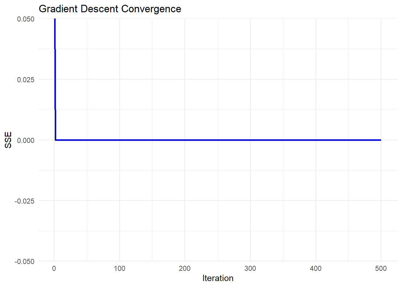

Figure 6.3: Gradient Descent Convergence

1. Steepest Descent (Gradient Descent) moves in the direction of steepest descent, which can lead to zigzagging behavior.
2. Slow convergence occurs when the curvature of the function varies significantly across dimensions.
3. Learning rate tuning is critical:

   • If too large, the algorithm diverges.

   • If too small, progress is very slow.

4. Useful for initialization: It is often used to get close to the optimal solution before switching to more advanced methods like Gauss-Newton Algorithm or Newton’s method.

Several advanced techniques improve the performance of steepest descent:

• Momentum Gradient Descent: Adds a momentum term to smooth updates, reducing oscillations.

• Adaptive Learning Rates:

  • AdaGrad: Adjusts \(\alpha_j\) per parameter based on historical gradients.

  • RMSprop: Uses a moving average of past gradients to scale updates.

  • Adam (Adaptive Moment Estimation): Combines momentum and adaptive learning rates.

In practice, Adam is widely used in machine learning and deep learning, while Newton-based methods (including Gauss-Newton) are preferred for nonlinear regression.

---

6.2.1.4 Levenberg-Marquardt Algorithm

The Levenberg-Marquardt Algorithm is a widely used optimization method for solving nonlinear least squares problems. It is an adaptive technique that blends the Gauss-Newton Algorithm and Steepest Descent (Gradient Descent), dynamically switching between them based on problem conditions.

The update rule is:

\[ \hat{\theta}^{(j+1)} = \hat{\theta}^{(j)} - \alpha_j [\mathbf{F}(\hat{\theta}^{(j)})' \mathbf{F}(\hat{\theta}^{(j)}) + \tau \mathbf{I}_{p \times p}]\frac{\partial \mathbf{Q}(\hat{\theta}^{(j)})}{\partial \theta} \]

where:

• \(\tau\) is the damping parameter, controlling whether the step behaves like Gauss-Newton Algorithm or Steepest Descent (Gradient Descent).
• \(\mathbf{I}_{p \times p}\) is the identity matrix, ensuring numerical stability.
• \(\mathbf{F}(\hat{\theta}^{(j)})\) is the Jacobian matrix of partial derivatives.
• \(\frac{\partial \mathbf{Q}(\hat{\theta}^{(j)})}{\partial \theta}\) is the gradient vector.
• \(\alpha_j\) is the learning rate, determining step size.

The Levenberg-Marquardt algorithm is particularly useful when the Jacobian matrix \(\mathbf{F}(\hat{\theta}^{(j)})\) is nearly singular, meaning that Gauss-Newton Algorithm alone may fail.

• When \(\tau\) is large, the method behaves like Steepest Descent, ensuring stability.
• When \(\tau\) is small, it behaves like Gauss-Newton, accelerating convergence.
• Adaptive control of \(\tau\):
  • If \(SSE(\hat{\theta}^{(j+1)}) < SSE(\hat{\theta}^{(j)})\), reduce \(\tau\): \[ \tau \gets \tau / 10 \]
  • Otherwise, increase \(\tau\) to stabilize: \[ \tau \gets 10\tau \]

This adjustment ensures that the algorithm moves efficiently while avoiding instability.

# Load required libraries
library(minpack.lm)
library(ggplot2)

# Define a nonlinear function (exponential model)
nonlinear_model <- function(theta, x) {
    theta[1] * exp(theta[2] * x)
}

# Define SSE function
sse <- function(theta, x, y) {
    sum((y - nonlinear_model(theta, x)) ^ 2)
}

# Generate synthetic data
set.seed(123)
x <- seq(0, 10, length.out = 100)
true_theta <- c(2, 0.3)
y <- nonlinear_model(true_theta, x) + rnorm(length(x), sd = 0.5)

# Robust Levenberg-Marquardt Optimization Implementation
levenberg_marquardt <-
    function(theta_init,
             x,
             y,
             tol = 1e-6,
             max_iter = 500,
             tau_init = 1) {
        theta <- theta_init
        tau <- tau_init
        lambda <- 1e-8  # Small regularization term
        sse_values <- numeric(max_iter)
        
        for (j in 1:max_iter) {
            # Compute Jacobian matrix numerically
            epsilon <- 1e-6
            F_matrix <-
                matrix(0, nrow = length(y), ncol = length(theta))
            for (p in 1:length(theta)) {
                theta_perturb <- theta
                theta_perturb[p] <- theta[p] + epsilon
                F_matrix[, p] <-
                    (nonlinear_model(theta_perturb, x) 
                     - nonlinear_model(theta, x)) / epsilon
            }
            
            # Compute residuals
            residuals <- y - nonlinear_model(theta, x)
            
            # Compute Levenberg-Marquardt update
            A <-
                t(F_matrix) %*% F_matrix + tau * diag(length(theta)) 
            + lambda * diag(length(theta))  # Regularized A
            delta <- tryCatch(
                solve(A) %*% t(F_matrix) %*% residuals,
                error = function(e) {
                    cat("Singular matrix detected at iteration",
                        j,
                        "- Increasing tau\n")
                    tau <<- tau * 10  # Increase tau to stabilize
                    # Return zero delta to avoid NaN updates
                    return(rep(0, length(theta)))  
                }
            )
            
            theta_new <- theta + delta
            
            # Compute new SSE
            sse_values[j] <- sse(theta_new, x, y)
            
            # Adjust tau dynamically
            if (sse_values[j] < sse(theta, x, y)) {
                # Reduce tau but prevent it from going too low
                tau <-
                    max(tau / 10, 1e-8)  
            } else {
                tau <- tau * 10  # Increase tau if SSE increases
            }
            
            # Check for convergence
            if (sum(abs(delta)) < tol) {
                cat("Converged in", j, "iterations.\n")
                return(list(theta = theta_new, sse_values = sse_values[1:j]))
            }
            
            theta <- theta_new
        }
        
        return(list(theta = theta, sse_values = sse_values))
    }

# Run Levenberg-Marquardt
theta_init <- c(1, 0.1)  # Initial guess
result <- levenberg_marquardt(theta_init, x, y)
#> Singular matrix detected at iteration 11 - Increasing tau
#> Converged in 11 iterations.

# Extract results
estimated_theta <- result$theta
sse_values <- result$sse_values

# Display estimated parameters
cat("Estimated parameters (A, B) using Levenberg-Marquardt:\n")
#> Estimated parameters (A, B) using Levenberg-Marquardt:
print(estimated_theta)
#>               [,1]
#> [1,] -6.473440e-09
#> [2,]  1.120637e+01

# Plot convergence of SSE over iterations
sse_df <-
    data.frame(Iteration = seq_along(sse_values), SSE = sse_values)

ggplot(sse_df, aes(x = Iteration, y = SSE)) +
    geom_line(color = "blue", linewidth = 1) +
    labs(title = "Levenberg-Marquardt Convergence",
         x = "Iteration",
         y = "SSE") +
    theme_minimal()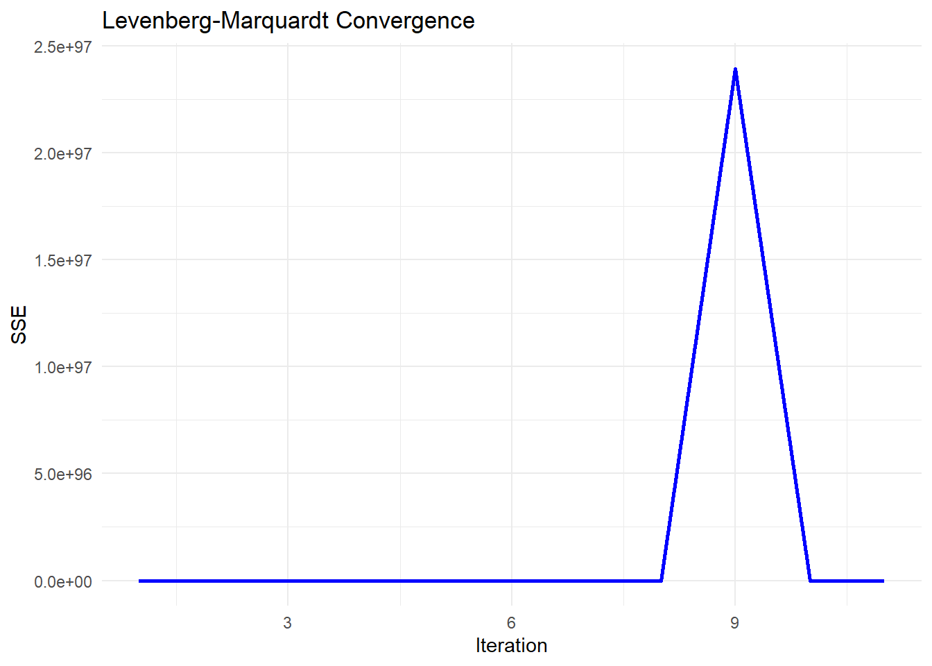

Figure 6.4: Levenberg–Marquardt Convergence

• Early Stability (Flat SSE)

  • The SSE remains near zero for the first few iterations, which suggests that the algorithm is initially behaving stably.

  • This might indicate that the initial parameter guess is reasonable, or that the updates are too small to significantly affect SSE.

• Sudden Explosion in SSE (Iteration ~8-9)

  • The sharp spike in SSE at iteration 9 indicates a numerical instability or divergence in the optimization process.

  • This could be due to:

    • An ill-conditioned Jacobian matrix: The step direction is poorly estimated, leading to an unstable jump.

    • A sudden large update (delta): The damping parameter (tau) might have been reduced too aggressively, causing an uncontrolled step.

    • Floating-point issues: If A becomes nearly singular, solving A \ delta = residuals may produce excessively large values.

• Return to Stability (After Iteration 9)

  • The SSE immediately returns to a low value after the spike, which suggests that the damping parameter (tau) might have been increased after detecting instability.

  • This is consistent with the adaptive nature of Levenberg-Marquardt:

    • If a step leads to a bad SSE increase, the algorithm increases tau to make the next step more conservative.

    • If the next step stabilizes, tau may be reduced again.

6.2.1.5 Newton-Raphson Algorithm

The Newton-Raphson method is a second-order optimization technique used for nonlinear least squares problems. Unlike first-order methods (such as Steepest Descent (Gradient Descent) and Gauss-Newton Algorithm), Newton-Raphson uses both first and second derivatives of the objective function for faster convergence.

The update rule is:

\[ \hat{\theta}^{(j+1)} = \hat{\theta}^{(j)} - \alpha_j \left[\frac{\partial^2 Q(\hat{\theta}^{(j)})}{\partial \theta \partial \theta'}\right]^{-1} \frac{\partial Q(\hat{\theta}^{(j)})}{\partial \theta} \]

where:

• \(\frac{\partial Q(\hat{\theta}^{(j)})}{\partial \theta}\) is the gradient vector (first derivative of the objective function).
• \(\frac{\partial^2 Q(\hat{\theta}^{(j)})}{\partial \theta \partial \theta'}\) is the Hessian matrix (second derivative of the objective function).
• \(\alpha_j\) is the learning rate, controlling step size.

The Hessian matrix in nonlinear least squares problems is:

\[ \frac{\partial^2 Q(\hat{\theta}^{(j)})}{\partial \theta \partial \theta'} = 2 \mathbf{F}(\hat{\theta}^{(j)})' \mathbf{F}(\hat{\theta}^{(j)}) - 2\sum_{i=1}^{n} [Y_i - f(x_i;\theta)] \frac{\partial^2 f(x_i;\theta)}{\partial \theta \partial \theta'} \]

where:

• The first term \(2 \mathbf{F}(\hat{\theta}^{(j)})' \mathbf{F}(\hat{\theta}^{(j)})\) is the same as in the Gauss-Newton Algorithm.
• The second term \(-2\sum_{i=1}^{n} [Y_i - f(x_i;\theta)] \frac{\partial^2 f(x_i;\theta)}{\partial \theta \partial \theta'}\) contains second-order derivatives.

Key Observations

• Gauss-Newton vs. Newton-Raphson:
  • Gauss-Newton approximates the Hessian by ignoring the second term.
  • Newton-Raphson explicitly incorporates second-order derivatives, making it more precise but computationally expensive.
• Challenges:
  • The Hessian matrix may be singular, making it impossible to invert.
  • Computing second derivatives is often difficult for complex functions.

# Load required libraries
library(ggplot2)

# Define a nonlinear function (exponential model)
nonlinear_model <- function(theta, x) {
    theta[1] * exp(theta[2] * x)
}

# Define SSE function
sse <- function(theta, x, y) {
    sum((y - nonlinear_model(theta, x)) ^ 2)
}

# Compute Gradient (First Derivative) of SSE
gradient_sse <- function(theta, x, y) {
    residuals <- y - nonlinear_model(theta, x)
    
    # Partial derivative w.r.t theta_1
    grad_1 <- -2 * sum(residuals * exp(theta[2] * x))
    
    # Partial derivative w.r.t theta_2
    grad_2 <- -2 * sum(residuals * theta[1] * x * exp(theta[2] * x))
    
    return(c(grad_1, grad_2))
}

# Compute Hessian (Second Derivative) of SSE
hessian_sse <- function(theta, x, y) {
    residuals <- y - nonlinear_model(theta, x)
    
    # Compute second derivatives
    H_11 <- 2 * sum(exp(2 * theta[2] * x))
    H_12 <- 2 * sum(x * exp(2 * theta[2] * x) * theta[1])
    H_21 <- H_12
    
    term1 <- 2 * sum((x ^ 2) * exp(2 * theta[2] * x) * theta[1] ^ 2)
    term2 <- 2 * sum(residuals * (x ^ 2) * exp(theta[2] * x))
    
    H_22 <- term1 - term2
    
    return(matrix(
        c(H_11, H_12, H_21, H_22),
        nrow = 2,
        byrow = TRUE
    ))
}

# Generate synthetic data
set.seed(123)
x <- seq(0, 10, length.out = 100)
true_theta <- c(2, 0.3)
y <- nonlinear_model(true_theta, x) + rnorm(length(x), sd = 0.5)

# Newton-Raphson Optimization Implementation
newton_raphson <-
    function(theta_init,
             x,
             y,
             tol = 1e-6,
             max_iter = 500) {
        theta <- theta_init
        sse_values <- numeric(max_iter)
        
        for (j in 1:max_iter) {
            grad <- gradient_sse(theta, x, y)
            hessian <- hessian_sse(theta, x, y)
            
            # Check if Hessian is invertible
            if (det(hessian) == 0) {
                cat("Hessian is singular at iteration",
                    j,
                    "- Using identity matrix instead.\n")
                # Replace with identity matrix if singular
                hessian <-
                    diag(length(theta))  
            }
            
            # Compute Newton update
            delta <- solve(hessian) %*% grad
            theta_new <- theta - delta
            sse_values[j] <- sse(theta_new, x, y)
            
            # Check for convergence
            if (sum(abs(delta)) < tol) {
                cat("Converged in", j, "iterations.\n")
                return(list(theta = theta_new, sse_values = sse_values[1:j]))
            }
            
            theta <- theta_new
        }
        
        return(list(theta = theta, sse_values = sse_values))
    }

# Run Newton-Raphson
theta_init <- c(1, 0.1)  # Initial guess
result <- newton_raphson(theta_init, x, y)
#> Converged in 222 iterations.

# Extract results
estimated_theta <- result$theta
sse_values <- result$sse_values

# Display estimated parameters
cat("Estimated parameters (A, B) using Newton-Raphson:\n")
#> Estimated parameters (A, B) using Newton-Raphson:
print(estimated_theta)
#>           [,1]
#> [1,] 1.9934188
#> [2,] 0.3008742

# Plot convergence of SSE over iterations
sse_df <-
    data.frame(Iteration = seq_along(sse_values), SSE = sse_values)

ggplot(sse_df, aes(x = Iteration, y = SSE)) +
    geom_line(color = "blue", size = 1) +
    labs(title = "Newton-Raphson Convergence",
         x = "Iteration",
         y = "SSE") +
    theme_minimal()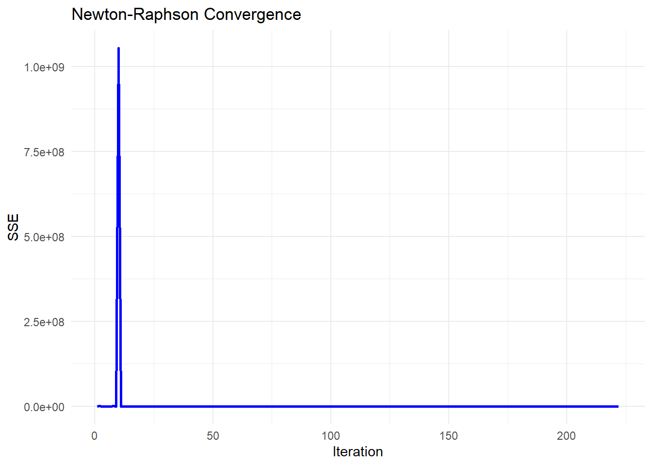

Figure 6.5: Newton–Raphson Convergence

6.2.1.6 Quasi-Newton Method

The Quasi-Newton method is an optimization technique that approximates Newton’s method without requiring explicit computation of the Hessian matrix. Instead, it iteratively constructs an approximation \(\mathbf{H}_j\) to the Hessian based on the first derivative information.

The update rule is:

\[ \hat{\theta}^{(j+1)} = \hat{\theta}^{(j)} - \alpha_j \mathbf{H}_j^{-1}\frac{\partial \mathbf{Q}(\hat{\theta}^{(j)})}{\partial \theta} \]

where:

• \(\mathbf{H}_j\) is a symmetric positive definite approximation to the Hessian matrix.
• As \(j \to \infty\), \(\mathbf{H}_j\) gets closer to the true Hessian.
• \(\frac{\partial Q(\hat{\theta}^{(j)})}{\partial \theta}\) is the gradient vector.
• \(\alpha_j\) is the learning rate, controlling step size.

Why Use Quasi-Newton Instead of Newton-Raphson Method?

• Newton-Raphson requires computing the Hessian matrix explicitly, which is computationally expensive and may be singular.
• Quasi-Newton avoids computing the Hessian directly by approximating it iteratively.
• Among first-order methods (which only require gradients, not Hessians), Quasi-Newton methods perform best.

---

Hessian Approximation

Instead of directly computing the Hessian \(\mathbf{H}_j\), Quasi-Newton methods update an approximation \(\mathbf{H}_j\) iteratively.

One of the most widely used formulas is the Broyden-Fletcher-Goldfarb-Shanno (BFGS) update:

\[ \mathbf{H}_{j+1} = \mathbf{H}_j + \frac{(\mathbf{s}_j \mathbf{s}_j')}{\mathbf{s}_j' \mathbf{y}_j} - \frac{\mathbf{H}_j \mathbf{y}_j \mathbf{y}_j' \mathbf{H}_j}{\mathbf{y}_j' \mathbf{H}_j \mathbf{y}_j} \]

where:

• \(\mathbf{s}_j = \hat{\theta}^{(j+1)} - \hat{\theta}^{(j)}\) (change in parameters).
• \(\mathbf{y}_j = \nabla Q(\hat{\theta}^{(j+1)}) - \nabla Q(\hat{\theta}^{(j)})\) (change in gradient).
• \(\mathbf{H}_j\) is the current inverse Hessian approximation.

---

# Load required libraries
library(ggplot2)

# Define a nonlinear function (exponential model)
nonlinear_model <- function(theta, x) {
    theta[1] * exp(theta[2] * x)
}

# Define SSE function
sse <- function(theta, x, y) {
    sum((y - nonlinear_model(theta, x))^2)
}

# Generate synthetic data
set.seed(123)
x <- seq(0, 10, length.out = 100)
true_theta <- c(2, 0.3)
y <- nonlinear_model(true_theta, x) + rnorm(length(x), sd = 0.5)

# Run BFGS Optimization using `optim()`
theta_init <- c(1, 0.1)  # Initial guess
result <- optim(
    par = theta_init,
    fn = function(theta) sse(theta, x, y),  # Minimize SSE
    method = "BFGS",
    control = list(trace = 0)  # Suppress optimization progress
    # control = list(trace = 1, REPORT = 1)  # Print optimization progress
)

# Extract results
estimated_theta <- result$par
sse_final <- result$value
convergence_status <- result$convergence  # 0 means successful convergence

# Display estimated parameters
cat("\n=== Optimization Results ===\n")
#> 
#> === Optimization Results ===
cat("Estimated parameters (A, B) using Quasi-Newton BFGS:\n")
#> Estimated parameters (A, B) using Quasi-Newton BFGS:
print(estimated_theta)
#> [1] 1.9954216 0.3007569

# Display final SSE
cat("\nFinal SSE:", sse_final, "\n")
#> 
#> Final SSE: 20.3227

6.2.1.7 Trust-Region Reflective Algorithm

The Trust-Region Reflective (TRR) algorithm is an optimization technique used for nonlinear least squares problems. Unlike Newton’s method and gradient-based approaches, TRR dynamically restricts updates to a trust region, ensuring stability and preventing overshooting.

The goal is to minimize the objective function \(Q(\theta)\) (e.g., Sum of Squared Errors, SSE):

\[ \hat{\theta} = \arg\min_{\theta} Q(\theta) \]

Instead of taking a full Newton step, TRR solves the following quadratic subproblem:

\[ \min_{\delta} m_j(\delta) = Q(\hat{\theta}^{(j)}) + \nabla Q(\hat{\theta}^{(j)})' \delta + \frac{1}{2} \delta' \mathbf{H}_j \delta \]

subject to:

\[ \|\delta\| \leq \Delta_j \]

where:

• \(\mathbf{H}_j\) is an approximation of the Hessian matrix.

• \(\nabla Q(\hat{\theta}^{(j)})\) is the gradient vector.

• \(\Delta_j\) is the trust-region radius, which is adjusted dynamically.

---

Trust-Region Adjustments

The algorithm modifies the step size dynamically based on the ratio \(\rho_j\):

\[ \rho_j = \frac{Q(\hat{\theta}^{(j)}) - Q(\hat{\theta}^{(j)} + \delta)}{m_j(0) - m_j(\delta)} \]

• If \(\rho_j > 0.75\) and \(\|\delta\| = \Delta_j\), then expand the trust region: \[ \Delta_{j+1} = 2 \Delta_j \]

• If \(\rho_j < 0.25\), shrink the trust region: \[ \Delta_{j+1} = \frac{1}{2} \Delta_j \]

• If \(\rho_j > 0\), accept the step; otherwise, reject it.

If a step violates a constraint, it is reflected back into the feasible region:

\[ \hat{\theta}^{(j+1)} = \max(\hat{\theta}^{(j)} + \delta, \theta_{\min}) \]

This ensures that the optimization respects parameter bounds.

---

# Load required libraries
library(ggplot2)


# Define a nonlinear function (exponential model)
nonlinear_model <- function(theta, x) {
    theta[1] * exp(theta[2] * x)
}

# Define SSE function
sse <- function(theta, x, y) {
    sum((y - nonlinear_model(theta, x)) ^ 2)
}

# Compute Gradient (First Derivative) of SSE
gradient_sse <- function(theta, x, y) {
    residuals <- y - nonlinear_model(theta, x)
    
    # Partial derivative w.r.t theta_1
    grad_1 <- -2 * sum(residuals * exp(theta[2] * x))
    
    # Partial derivative w.r.t theta_2
    grad_2 <- -2 * sum(residuals * theta[1] * x * exp(theta[2] * x))
    
    return(c(grad_1, grad_2))
}

# Compute Hessian Approximation of SSE
hessian_sse <- function(theta, x, y) {
    residuals <- y - nonlinear_model(theta, x)
    
    # Compute second derivatives
    H_11 <- 2 * sum(exp(2 * theta[2] * x))
    H_12 <- 2 * sum(x * exp(2 * theta[2] * x) * theta[1])
    H_21 <- H_12
    
    term1 <- 2 * sum((x ^ 2) * exp(2 * theta[2] * x) * theta[1] ^ 2)
    term2 <- 2 * sum(residuals * (x ^ 2) * exp(theta[2] * x))
    
    H_22 <- term1 - term2
    
    return(matrix(
        c(H_11, H_12, H_21, H_22),
        nrow = 2,
        byrow = TRUE
    ))
}

# Generate synthetic data
set.seed(123)
x <- seq(0, 10, length.out = 100)
true_theta <- c(2, 0.3)
y <- nonlinear_model(true_theta, x) + rnorm(length(x), sd = 0.5)

# Manual Trust-Region Reflective Optimization Implementation
trust_region_reflective <-
    function(theta_init,
             x,
             y,
             tol = 1e-6,
             max_iter = 500,
             delta_max = 1.0) {
        theta <- theta_init
        delta_j <- 0.5  # Initial trust-region size
        n <- length(theta)
        sse_values <- numeric(max_iter)
        
        for (j in 1:max_iter) {
            grad <- gradient_sse(theta, x, y)
            hessian <- hessian_sse(theta, x, y)
            
            # Check if Hessian is invertible
            if (det(hessian) == 0) {
                cat("Hessian is singular at iteration",
                    j,
                    "- Using identity matrix instead.\n")
                hessian <-
                    diag(n)  # Replace with identity matrix if singular
            }
            
            # Compute Newton step
            delta_full <- -solve(hessian) %*% grad
            
            # Apply trust-region constraint
            if (sqrt(sum(delta_full ^ 2)) > delta_j) {
                # Scale step
                delta <-
                    (delta_j / sqrt(sum(delta_full ^ 2))) * delta_full  
            } else {
                delta <- delta_full
            }
            
            # Compute new theta and ensure it respects constraints
            theta_new <-
                pmax(theta + delta, c(0,-Inf))  # Reflect to lower bound
            sse_new <- sse(theta_new, x, y)
            
            # Compute agreement ratio (rho_j)
            predicted_reduction <-
                -t(grad) %*% delta - 0.5 * t(delta) %*% hessian %*% delta
            actual_reduction <- sse(theta, x, y) - sse_new
            rho_j <- actual_reduction / predicted_reduction
            
            # Adjust trust region size
            if (rho_j < 0.25) {
                delta_j <- max(delta_j / 2, 1e-4)  # Shrink
            } else if (rho_j > 0.75 &&
                       sqrt(sum(delta ^ 2)) == delta_j) {
                delta_j <- min(2 * delta_j, delta_max)  # Expand
            }
            
            # Accept or reject step
            if (rho_j > 0) {
                theta <- theta_new  # Accept step
            } else {
                cat("Step rejected at iteration", j, "\n")
            }
            
            sse_values[j] <- sse(theta, x, y)
            
            # Check for convergence
            if (sum(abs(delta)) < tol) {
                cat("Converged in", j, "iterations.\n")
                return(list(theta = theta, sse_values = sse_values[1:j]))
            }
        }
        
        return(list(theta = theta, sse_values = sse_values))
    }

# Run Manual Trust-Region Reflective Algorithm
theta_init <- c(1, 0.1)  # Initial guess
result <- trust_region_reflective(theta_init, x, y)

# Extract results
estimated_theta <- result$theta
sse_values <- result$sse_values

# Plot convergence of SSE over iterations
sse_df <-
    data.frame(Iteration = seq_along(sse_values), SSE = sse_values)

ggplot(sse_df, aes(x = Iteration, y = SSE)) +
    geom_line(color = "blue", size = 1) +
    labs(title = "Trust-Region Reflective Convergence",
         x = "Iteration",
         y = "SSE") +
    theme_minimal()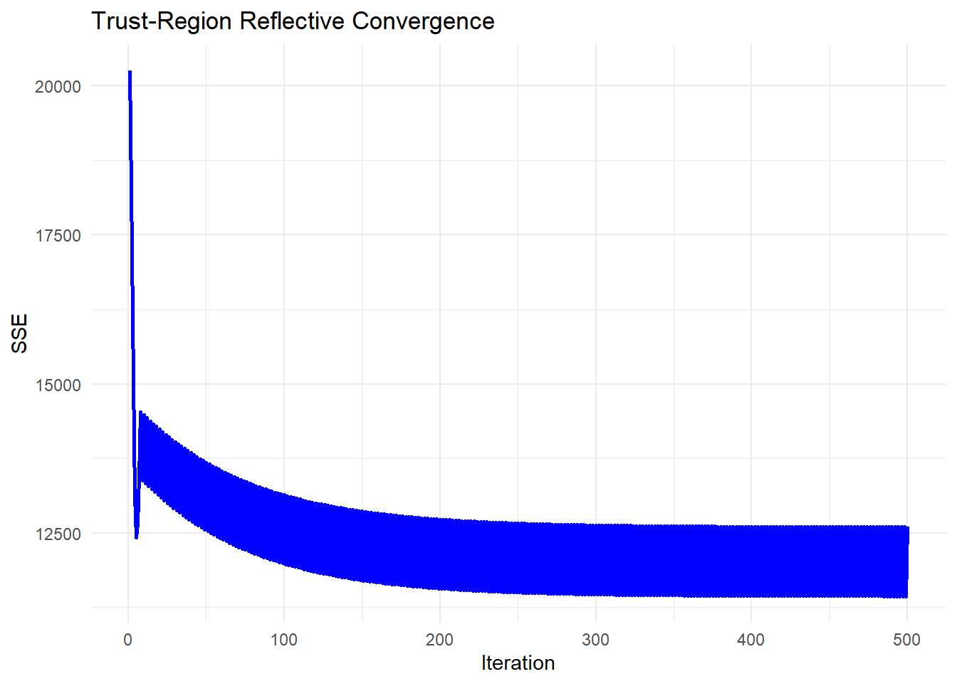

Figure 6.6: Trust-Region Reflective Convergence

---

This chapter is fully available in the published Springer volumes.
The online preview is limited per publisher guidelines.

To access the complete content, purchase the book on Springer:

Vol.	Title	Link
1	Foundations of Data Analysis	Buy on Springer
2	Regression Techniques for Data Analysis	Buy on Springer
3	Advanced Modeling and Data Challenges	Buy on Springer
4	Experimental Design	Buy on Springer

📖 Free preview — limited per publisher guidelines. Purchase the complete A Guide on Data Analysis series (Vols. 1–4) on Springer.

Vol. 1 Vol. 2 Vol. 3 Vol. 4