57.1 The Dynamic Optimization Problem

An agent observes a state and chooses an action in each period to maximize the expected present discounted value of a stream of payoffs. Let the action in period \(t\) be \(a_t \in \{0, 1, \dots, J\}\) and the state be \((x_t, \varepsilon_t)\), where \(x_t\) is a state observed by the econometrician and \(\varepsilon_t = (\varepsilon_{0t}, \dots, \varepsilon_{Jt})\) is a vector of choice-specific shocks observed by the agent but not the econometrician. The per-period payoff from choosing action \(a\) is

\[u(x_t, a) + \varepsilon_{a t},\]

additively separable in the observed flow utility \(u(x_t, a)\) and the private shock \(\varepsilon_{a t}\). The agent discounts the future at rate \(\beta \in (0, 1)\) and the observed state evolves according to a controlled Markov transition \(p(x_{t+1} \mid x_t, a_t)\). The agent’s problem is to choose a decision rule mapping states to actions that solves

\[ \max_{\{a_t\}} \; \mathbb{E} \left[ \sum_{\tau = t}^{\infty} \beta^{\tau - t} \big( u(x_\tau, a_\tau) + \varepsilon_{a_\tau \tau} \big) \,\middle|\, x_t, \varepsilon_t \right]. \]

57.2 Estimation by Nested Fixed Point

Rust (1987) estimated the structural parameters \(\theta = (\theta_1, R)\) by maximum likelihood, using the choice probabilities in equation (57.2) as the likelihood contributions. The complication is that those probabilities depend on the conditional value functions, which depend on the integrated value function, which is itself the solution of the fixed-point problem above and so depends on \(\theta\). The nested fixed point algorithm (NFXP) handles this with two nested loops.

The inner loop solves the agent’s dynamic program for a candidate parameter vector. Given \(\theta\) it iterates the Bellman operator

\[ \bar V(x) \;\leftarrow\; \gamma + \log \sum_{j} \exp\Big( u(x, j; \theta) + \beta \sum_{x'} \bar V(x') \, p(x' \mid x, j) \Big) \]

to convergence. Because the operator is a contraction with modulus \(\beta\), value-function iteration converges geometrically, and Rust’s original implementation accelerated the tail with Newton-Kantorovich steps. The fixed point delivers \(\bar V(\cdot; \theta)\) and hence the conditional value functions and the choice probabilities \(P(a \mid x; \theta)\).

The outer loop maximizes the log-likelihood of the observed panel of decisions \(\{a_{it}, x_{it}\}\) over \(\theta\),

\[ \ell(\theta) = \sum_{i} \sum_{t} \log P\big(a_{it} \mid x_{it}; \theta\big), \]

calling the inner loop afresh at every trial value of \(\theta\) proposed by the optimizer. The estimator is the full-solution maximum likelihood estimator: it is statistically efficient because it uses the exact model-implied likelihood, but it pays for that efficiency by solving the dynamic program many times. The transition probabilities \(p(x' \mid x, a)\) are usually estimated separately in a first step from the observed mileage increments, which do not depend on the utility parameters, so the likelihood that NFXP maximizes is a partial likelihood for \(\theta\) given the estimated transitions.

57.3 Conditional Choice Probability Estimation

The computational burden of repeatedly solving the dynamic program motivated a second tradition that avoids the full solution. The key insight, due to Hotz and Miller (1993), is that the structure of the model can be inverted: the differences in conditional value functions, which are what choices depend on, can be recovered directly from conditional choice probabilities that are observed in the data.

57.4 Finite Horizon, Discounting, and Identification

The infinite-horizon stationary model above is the most common setup, but many decisions have a natural terminal date: a worker nearing retirement, a patent nearing expiry, a student nearing graduation. In a finite-horizon model the value function carries a time subscript and is solved by backward induction from a known terminal value rather than by iterating a contraction. There is no fixed point to solve; one sweep from the last period to the first delivers the conditional value functions at every age, which is computationally easier but requires the analyst to specify the horizon and the terminal condition. CCP methods adapt naturally to finite horizons, since the backward recursion limits how far ahead the continuation values must reach.

A deeper issue is the identification of the discount factor \(\beta\). It is tempting to hope that forward-looking behavior reveals patience, but Magnac and Thesmar (2002) show that in the standard stationary dynamic discrete-choice model the discount factor is not identified from choice data alone. The intuition is a counting argument: the conditional choice probabilities at each state pin down the value differences, but for any fixed \(\beta\) there exists a flow-utility function that rationalizes those same probabilities exactly, so \(\beta\) and the per-period payoffs are observationally equivalent. Identification of \(\beta\) therefore requires outside information: an exclusion restriction in the form of a state variable that shifts the continuation value without entering the current flow utility, a known value for some payoff, or variation in the choice set across states. Applied work that estimates \(\beta\) rather than fixing it leans on exactly such restrictions, and work that fixes \(\beta\) at a calibrated value, commonly near \(0.95\) at annual frequency, is implicitly acknowledging this nonidentification. The lesson generalizes: the discount factor is the parameter most fragile to the model’s maintained assumptions, and its treatment should always be stated explicitly.

57.5 A Runnable Bus Engine Example

The following code implements a deliberately small version of the Rust model in base R. The state space is a coarse mileage grid, the dynamic program is solved by value-function iteration on the integrated value function, a panel of decisions is simulated from the implied choice probabilities, and the structural parameters are then recovered by nested fixed point maximum likelihood. Keeping the grid small lets the whole pipeline, solve, simulate, and estimate, run in a few seconds.

We begin with the primitives. Mileage is discretized into a grid of states; when the engine is kept it advances by zero, one, or two grid cells with fixed probabilities, and when it is replaced the state resets to the first cell before advancing.

set.seed(2024)

# State space: discretized mileage.
n_states <- 90L
states   <- 0:(n_states - 1L)

# True structural parameters.
theta1_true <- 0.05   # per-state operating cost slope
R_true      <- 4.00   # lump-sum replacement cost
beta        <- 0.95   # discount factor (fixed, not estimated)

# Mileage transition when the engine is KEPT: advance by 0, 1, or 2 cells.
trans_p <- c(0.30, 0.50, 0.20)

# Build the keep-transition matrix, absorbing at the top of the grid.
build_keep_matrix <- function(n_states, trans_p) {
    P <- matrix(0, n_states, n_states)
    for (s in 1:n_states) {
        for (k in seq_along(trans_p)) {
            s_next <- min(s + (k - 1L), n_states)
            P[s, s_next] <- P[s, s_next] + trans_p[k]
        }
    }
    P
}
P_keep <- build_keep_matrix(n_states, trans_p)

The flow utilities are negative costs: keeping the engine costs theta1 per unit of mileage, while replacing it costs the lump sum R. The integrated value function is found by iterating the log-sum Bellman operator to convergence. Replacement regenerates the state to the first grid cell, so its continuation value uses the first row of the keep-transition matrix.

# Solve the integrated value function by value-function iteration.
solve_vfi <- function(theta1, R, beta, P_keep, states,
                      tol = 1e-10, max_iter = 1000L) {
    n   <- length(states)
    EV  <- numeric(n)             # integrated value bar V(x)
    eul <- 0.5772156649           # Euler's constant

    # Flow utilities (negative costs).
    u_keep    <- -theta1 * states
    u_replace <- rep(-R, n)

    for (iter in 1:max_iter) {
        # Conditional value functions v(x, a).
        v_keep    <- u_keep    + beta * (P_keep %*% EV)
        # Replacement resets to state 1, then mileage advances from there.
        v_replace <- u_replace + beta * as.numeric(P_keep[1, ] %*% EV)

        # Log-sum gives the updated integrated value.
        m      <- pmax(v_keep, v_replace)        # for numerical stability
        EV_new <- eul + m + log(exp(v_keep - m) + exp(v_replace - m))
        EV_new <- as.numeric(EV_new)

        if (max(abs(EV_new - EV)) < tol) { EV <- EV_new; break }
        EV <- EV_new
    }

    v_keep    <- as.numeric(u_keep    + beta * (P_keep %*% EV))
    v_replace <- as.numeric(u_replace + beta * (P_keep[1, ] %*% EV))
    # Replacement (a = 1) probability via binary logit on value difference.
    p_replace <- 1 / (1 + exp(v_keep - v_replace))
    list(EV = EV, v_keep = v_keep, v_replace = v_replace,
         p_replace = p_replace)
}

sol <- solve_vfi(theta1_true, R_true, beta, P_keep, states)

The solution yields the replacement hazard, the conditional probability of replacing the engine at each mileage state. It is the empirical analogue of the hazard that Rust (1987) reports for Zurcher’s fleet, and as economic intuition demands it rises with mileage: the more worn the engine, the likelier replacement. Figure 57.1 plots this hazard against accumulated mileage.

library(ggplot2)

haz_df <- data.frame(mileage = states, p_replace = sol$p_replace)

ggplot(haz_df, aes(mileage, p_replace)) +
    geom_line(linewidth = 0.8, colour = "#2c3e50") +
    labs(x = "Mileage state",
         y = "Replacement probability",
         title = "Conditional choice probability of engine replacement") +
    causalverse::ama_theme()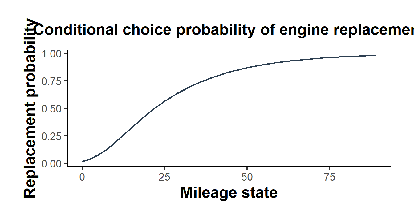

Figure 57.1: Replacement hazard from the solved bus engine model. The conditional probability of replacing the engine rises with accumulated mileage, since higher operating costs make the lump-sum replacement cost worth paying.

With the model solved we simulate a panel of buses. Each bus is followed over time; in every period it replaces or keeps according to the model’s choice probability, and mileage then evolves under the corresponding transition.

# Simulate a panel of N buses over T periods from the solved model.
simulate_panel <- function(sol, P_keep, n_states, N = 200L, Tt = 60L) {
    state  <- integer(N * Tt)
    action <- integer(N * Tt)
    trans_support <- 0:(length(trans_p) - 1L)

    for (i in 1:N) {
        s <- 1L  # all buses start with a fresh engine
        for (t in 1:Tt) {
            idx <- (i - 1L) * Tt + t
            # Draw the replacement decision.
            a <- as.integer(runif(1) < sol$p_replace[s])
            state[idx]  <- s
            action[idx] <- a
            # State next period: replacement resets to cell 1 first.
            base   <- if (a == 1L) 1L else s
            step   <- sample(trans_support, 1, prob = trans_p)
            s      <- min(base + step, n_states)
        }
    }
    data.frame(bus = rep(1:N, each = Tt), state = state, action = action)
}

panel <- simulate_panel(sol, P_keep, n_states, N = 200L, Tt = 60L)
mean(panel$action)   # fraction of periods with a replacement
#> [1] 0.098

Estimation by nested fixed point follows. The outer loop searches over the structural parameters; for each candidate the inner loop calls solve_vfi to obtain the choice probabilities, and the negative log-likelihood of the observed actions is returned to the optimizer. The transition probabilities are treated as known here, mirroring the usual first-step estimation of the mileage process.

# Negative log-likelihood: inner loop solves the dynamic program.
neg_loglik <- function(par, panel, beta, P_keep, states) {
    theta1 <- exp(par[1])   # exp keeps parameters positive
    R      <- exp(par[2])
    sol    <- solve_vfi(theta1, R, beta, P_keep, states)

    p_rep  <- sol$p_replace[panel$state]
    p_obs  <- ifelse(panel$action == 1L, p_rep, 1 - p_rep)
    p_obs  <- pmin(pmax(p_obs, 1e-12), 1 - 1e-12)
    -sum(log(p_obs))
}

# Outer loop: maximize the likelihood (minimize the negative).
fit <- optim(par = log(c(0.02, 2.0)), fn = neg_loglik,
             panel = panel, beta = beta, P_keep = P_keep, states = states,
             method = "Nelder-Mead",
             control = list(reltol = 1e-10, maxit = 500))

theta1_hat <- exp(fit$par[1])
R_hat      <- exp(fit$par[2])

The estimates recover the parameters that generated the data. The table juxtaposes the true and estimated values; sampling variation aside, the nested fixed point estimator returns the data-generating primitives.

results <- data.frame(
    Parameter = c("Operating cost slope ($\\theta_1$)",
                  "Replacement cost ($R$)"),
    True      = c(theta1_true, R_true),
    Estimated = c(theta1_hat, R_hat)
)

knitr::kable(results, digits = 3, escape = FALSE,
             caption = "True versus nested-fixed-point estimates of the bus engine structural parameters. The discount factor is fixed at 0.95 and the mileage transition probabilities are treated as known.")

As a lightweight check on the conditional-choice-probability logic, we can recover value differences without ever solving the dynamic program a second time. The Hotz-Miller inversion in equation (57.4) maps the empirical replacement frequency at a state directly into the difference \(v(x, 1) - v(x, 0)\), which lines up with the model-implied value difference used to generate the data. This is the first step of any CCP estimator: the smooth empirical CCPs stand in for the inner-loop solve.

# Empirical CCPs by state, lightly smoothed (Laplace), then Hotz-Miller.
n_rep   <- tapply(panel$action, panel$state, sum)
n_obs   <- tapply(panel$action, panel$state, length)
emp_states <- as.integer(names(n_obs))          # states seen in the data
p_hat   <- (as.numeric(n_rep) + 1) / (as.numeric(n_obs) + 2)

# Hotz-Miller: log P(replace) - log P(keep) = v(x,1) - v(x,0).
vdiff_ccp   <- log(p_hat) - log(1 - p_hat)
vdiff_model <- (sol$v_replace - sol$v_keep)[emp_states + 1L]

# Correlation between CCP-inverted and model value differences.
round(cor(vdiff_ccp, vdiff_model), 3)
#> [1] 0.969

The near-perfect correlation confirms that the choice frequencies encode the value differences, which is precisely why CCP methods can bypass the repeated dynamic programming solve that NFXP performs. In a full CCP estimator these inverted value differences would feed a forward-simulation step in the manner of Hotz et al. (1994) and a second-stage minimization over the structural parameters, exchanging a small efficiency loss for a large computational saving.

57.6 Practical Notes

A few points recur in applied work. The transition probabilities are almost always estimated in a first step, both because the mileage process does not depend on the utility parameters and because doing so shrinks the dimension of the outer optimization. The discount factor should be fixed unless an explicit exclusion restriction identifies it, in line with the Magnac and Thesmar (2002) nonidentification result. Numerical care in the inner loop matters: the log-sum should be computed with the max-subtraction trick used above to avoid overflow, and the value-function iteration tolerance should be tighter than the outer optimizer tolerance so that inner-loop error does not masquerade as a likelihood gradient. Finally, the choice between NFXP and CCP is a choice about scale. For the two-action, ninety-state problem here the full solution is instant and NFXP is the natural tool, but as the state space grows, as players are added, or as unobserved heterogeneity enters through the Arcidiacono and Miller (2011) finite-mixture EM machinery, the CCP route becomes not just convenient but necessary. The broader survey by Aguirregabiria and Mira (2010) maps these tradeoffs across the full landscape of estimators and is the standard entry point for the literature.