59.1 The Generalized Roy Model

The Roy model is the canonical economic account of self-selection. Each agent possesses two potential outcomes, one in each of two sectors, and chooses the sector that yields the higher net return. Because the choice depends on the potential outcomes themselves, the observed distribution in each sector is a selected, not a random, sample of the population. Heckman and Honoré (1990) characterized exactly what features of the joint distribution of potential outcomes can be recovered from such selected data, a question of empirical content that anchors everything that follows.

Let each agent have potential outcomes \(Y_1\) in sector or treatment state \(1\) and \(Y_0\) in state \(0\),

\[ Y_1 = \mu_1(X) + U_1, \qquad Y_0 = \mu_0(X) + U_0, \]

where \(X\) collects observed covariates and \((U_1, U_0)\) are unobservables with mean zero. The individual gain is \(Y_1 - Y_0 = \mu_1(X) - \mu_0(X) + (U_1 - U_0)\). The crucial term is \(U_1 - U_0\), the idiosyncratic component of the gain. In the original Roy model the agent chooses sector \(1\) whenever \(Y_1 > Y_0\), so selection is driven directly by the gain. The generalized Roy model adds a cost of choosing sector \(1\), which may depend on observed shifters \(Z\) and on its own unobservable,

\[ C = \mu_C(Z) + U_C, \]

and the agent selects \(D = 1\) when the net gain is positive,

\[ D = \mathbf{1}\{ Y_1 - Y_0 - C \ge 0 \} = \mathbf{1}\{ \mu_1(X) - \mu_0(X) - \mu_C(Z) + (U_1 - U_0 - U_C) \ge 0 \}. \]

Two regimes of this model deserve separate names. Under selection on levels, the unobservable governing choice is uncorrelated with the gain \(U_1 - U_0\), so that treatment effects are homogeneous in the unobservables and the various average parameters coincide. Under selection on gains, also called essential heterogeneity, the term \(U_1 - U_0\) enters the choice rule with nonzero correlation, meaning agents act on private information about their own returns. This is the case that breaks the equality of the average parameters and that the rest of the chapter is built to handle (Heckman and Vytlacil 2005).

The connection to the Heckman selection model is direct. That model is the special case in which \(Y_0\) is never observed, so only the sector-\(1\) outcome equation and the selection index appear, and the inverse Mills ratio corrects the conditional mean of \(Y_1\) given \(D = 1\). The generalized Roy model observes outcomes in both states and therefore lets us recover both margins and, with sufficient variation, the distribution of gains. The cost shifters \(Z\) that enter the choice equation but are excluded from the outcome equations play the role of instruments: they move the probability of selection without directly moving the potential outcomes.

n <- 20000

# Observed covariate and an excluded cost shifter (the instrument)
X <- rnorm(n)
Z <- rnorm(n)

# Latent gain component shared by the outcome and the choice rule
gain_u <- rnorm(n)              # private knowledge of idiosyncratic gain
U0     <- 0.5 * rnorm(n)        # baseline-state noise
noise1 <- 0.5 * rnorm(n)

# Potential outcomes: the gain loads positively on gain_u
Y0 <- 1.0 + 0.8 * X + U0
Y1 <- 1.6 + 1.0 * X + 1.2 * gain_u + noise1
gain <- Y1 - Y0                 # individual treatment effect

# Choice: agents act on the gain (essential heterogeneity) and on cost shifter Z
cost  <- 0.4 - 0.7 * Z
index <- gain - cost + 0.3 * rnorm(n)
D <- as.integer(index >= 0)

Yobs <- D * Y1 + (1 - D) * Y0

ATE <- mean(gain)
TT  <- mean(gain[D == 1])
OLS <- coef(lm(Yobs ~ D + X))["D"]

roy_tab <- data.frame(
  Parameter = c("OLS (naive)", "ATE", "TT (effect on treated)"),
  Value     = round(c(OLS, ATE, TT), 3)
)
roy_tab
#>                Parameter Value
#> 1            OLS (naive) 1.217
#> 2                    ATE 0.596
#> 3 TT (effect on treated) 1.492

59.2 Marginal Treatment Effects

Heckman and Vytlacil (2005) introduced the marginal treatment effect (MTE) as the fundamental building block from which every conventional treatment parameter can be assembled. Write the choice equation as a latent index crossing a threshold,

\[ D = \mathbf{1}\{ \mu_D(Z) - V \ge 0 \}, \]

where \(V\) collects the unobservables in the choice rule, normalized so that \(P(Z) \equiv \Pr(D = 1 \mid Z)\), the propensity score, equals the rank of \(-V\) in its own distribution. Define \(U_D = F_V(V)\), the quantile of the choice unobservable, which lives on the unit interval. An agent participates when \(P(Z) \ge U_D\). A small \(U_D\) marks an agent eager to participate, one who selects in even when the observed inducement is weak; a large \(U_D\) marks a reluctant agent who participates only when \(P(Z)\) is near one.

The MTE is the average gain for agents at the margin of indifference at a given value of the choice unobservable,

\[ \text{MTE}(x, u) = \mathbb{E}\!\left[ Y_1 - Y_0 \mid X = x,\, U_D = u \right]. \]

Reading across \(u\) traces out how the gain varies with unobserved resistance to treatment. Under essential heterogeneity the MTE slopes: agents with low \(U_D\), who select in readily, have systematically different gains from agents with high \(U_D\), who must be pushed in. A flat MTE is the visible signature of the absence of selection on gains, since then the marginal and average agents are alike.

59.2.2 Local Instrumental Variables Estimation

The MTE is identified by local instrumental variables (LIV). The key identity is that the conditional expectation of the observed outcome, given covariates and the propensity score, has a derivative in the propensity score equal to the MTE,

\[ \frac{\partial}{\partial p}\, \mathbb{E}\!\left[ Y \mid X = x,\, P(Z) = p \right] = \text{MTE}(x, p). \]

Intuitively, nudging the propensity score from \(p\) to \(p + dp\) draws in exactly the agents whose choice unobservable \(U_D\) sits at \(p\), so the resulting change in mean outcome reveals their average gain. Estimation proceeds in two steps. First fit the propensity score, typically a probit or logit of \(D\) on \(Z\) and \(X\). Then regress the outcome flexibly on the fitted propensity score and differentiate, either by fitting a polynomial in \(p\) and taking its analytic derivative or by local polynomial smoothing. Carneiro et al. (2011) implemented this program to estimate the marginal return to a college education and found the return to fall as the unobserved resistance to schooling rises, the empirical face of selection on gains.

We illustrate with a deliberately simple LIV estimator: fit the propensity score, then fit a low-order polynomial of the outcome in the estimated propensity score and read off the slope as the MTE.

n <- 8000

# Two instruments shift the propensity score over a wide range
Z1 <- rnorm(n); Z2 <- rnorm(n)

# Choice unobservable on the latent index scale
V  <- rnorm(n)

# Latent index and binary choice
idx <- 0.3 + 0.9 * Z1 + 0.9 * Z2
D   <- as.integer(idx - V >= 0)

# Essential heterogeneity: the gain declines in the choice unobservable V.
# Agents with small V (eager, low U_D) enjoy larger gains.
b0 <- 1.0
gain_i <- 2.0 - 1.4 * V             # individual gain falls with V
Y0 <- b0 + 0.5 * rnorm(n)
Y1 <- Y0 + gain_i
Y  <- D * Y1 + (1 - D) * Y0

# Step 1: propensity score via probit on the instruments
ps_fit <- glm(D ~ Z1 + Z2, family = binomial("probit"))
phat   <- predict(ps_fit, type = "response")

# Step 2: flexible regression of Y on the propensity score; the derivative is the MTE
poly_fit <- lm(Y ~ phat + I(phat^2) + I(phat^3))
cf <- coef(poly_fit)

grid <- seq(0.05, 0.95, by = 0.01)
# d/dp of (b1 p + b2 p^2 + b3 p^3) = b1 + 2 b2 p + 3 b3 p^2
mte_hat <- cf["phat"] + 2 * cf["I(phat^2)"] * grid + 3 * cf["I(phat^3)"] * grid^2

# True MTE on the U_D = Phi(V) scale: with gain = 2 - 1.4 V and U_D = Phi(V),
# we have V = qnorm(U_D), so MTE(u) = 2 - 1.4 * qnorm(u)
mte_true <- 2.0 - 1.4 * qnorm(grid)

mte_df <- data.frame(
  u        = grid,
  estimate = mte_hat,
  truth    = mte_true
)
head(mte_df, 4)
#>      u estimate    truth
#> 1 0.05 3.480416 4.302795
#> 2 0.06 3.470928 4.176683
#> 3 0.07 3.460646 4.066107
#> 4 0.08 3.449567 3.967100

The estimated and true curves both slope downward in \(u\), confirming that the eager agents at low \(u\) carry the larger gains. Figure 59.1 overlays the two and adds the aggregation weights for the ATE and the effect on the treated, so the geometry of the parameters is visible alongside the curve itself.

library(ggplot2)

# Illustrative TT weights: proportional to the share of agents with U_D <= u
w_ate <- rep(1, length(grid))
w_tt  <- (1 - grid)
w_tt  <- w_tt / mean(w_tt)        # normalize to mean 1 for comparability

plot_df <- rbind(
  data.frame(u = grid, value = mte_df$truth,    series = "MTE (true)"),
  data.frame(u = grid, value = mte_df$estimate, series = "MTE (LIV estimate)"),
  data.frame(u = grid, value = w_ate,           series = "Weight: ATE"),
  data.frame(u = grid, value = w_tt,            series = "Weight: TT")
)

ggplot(plot_df, aes(u, value, color = series, linetype = series)) +
  geom_line(linewidth = 0.9) +
  labs(
    x = "Unobserved resistance to treatment, u = U_D",
    y = "MTE   /   aggregation weight",
    color = NULL, linetype = NULL
  ) +
  causalverse::ama_theme()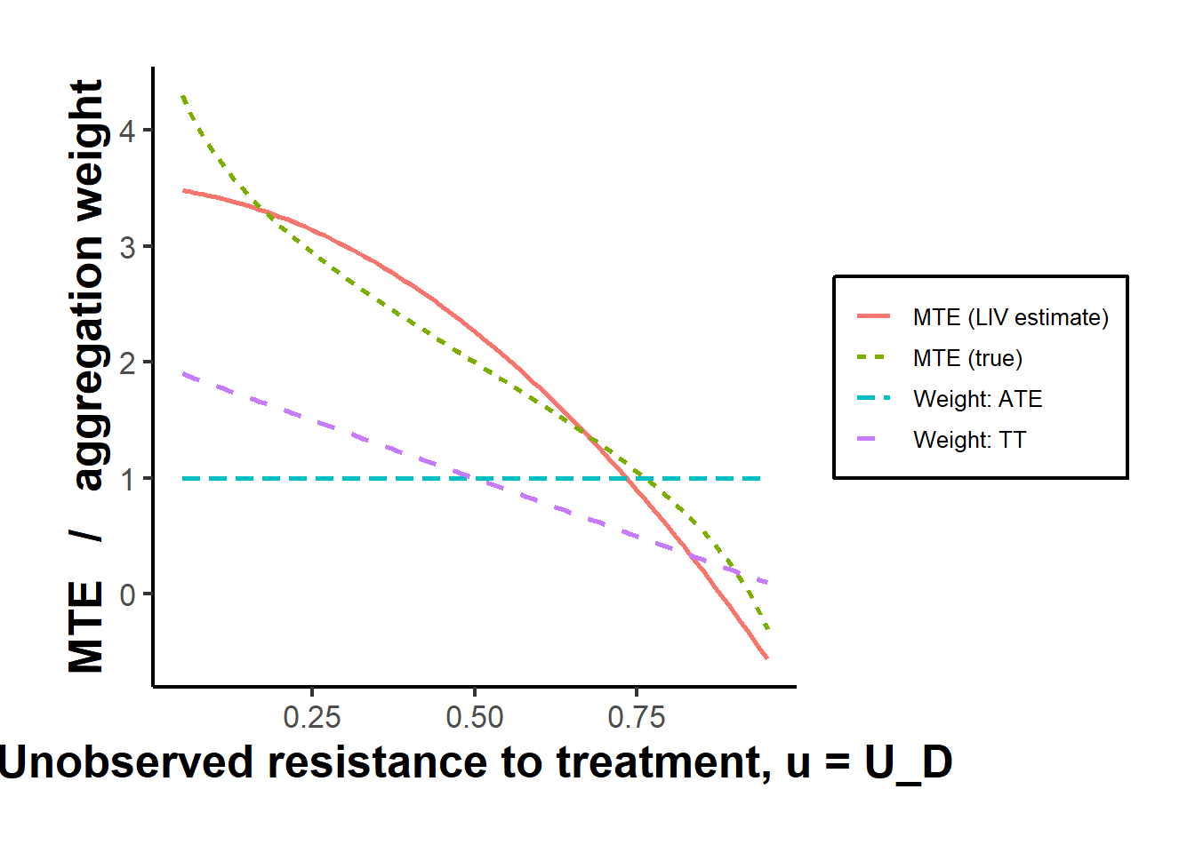

Figure 59.1: Estimated and true marginal treatment effect as a function of the unobserved resistance to treatment \(u = U_D\), together with the aggregation weights that map the curve into the average treatment effect (uniform) and the effect on the treated (declining). Because the curve slopes, the two parameters diverge.

The LIV estimate tracks the true MTE over the interior of the support, with the usual degradation near the boundaries where the propensity score is rarely observed and the polynomial extrapolates. The ATE weight is flat, so the ATE is the simple area under the curve, whereas the TT weight tilts toward the eager low-\(u\) agents, which is why the effect on the treated lands above the average. The picture makes concrete the claim that the parameters are weighted averages of a single underlying object.

59.3 Unobserved Heterogeneity via Finite Mixtures

The Roy and MTE frameworks treat the choice unobservable as continuous. A complementary tradition models unobserved heterogeneity as a small number of discrete latent types, each with its own parameters, and lets the data infer both the type-specific parameters and the population shares. This is the finite mixture approach, and it is workhorse machinery in the structural literature on dynamic discrete choice, where unobserved types capture persistent heterogeneity in preferences or costs that would otherwise be confounded with state dependence. The treatment here is the static, cross-sectional version; the dynamic extension that carries types through a sequence of choices is developed in the chapter on dynamic discrete choice.

Suppose the population is a mixture of \(K\) types with shares \(\pi_1, \dots, \pi_K\) summing to one. Conditional on belonging to type \(k\), an outcome \(y\) is drawn from a density \(f(y \mid \theta_k)\). The observed density is the mixture

\[ f(y) = \sum_{k=1}^{K} \pi_k\, f(y \mid \theta_k). \]

Type membership is latent, so the likelihood does not factor into a clean per-type form. The EM algorithm resolves this by alternating between a step that computes, for each observation, the posterior probability of belonging to each type given current parameters, and a step that updates the parameters as if those posterior probabilities were known weights. The posterior responsibility of type \(k\) for observation \(i\) is

\[ \gamma_{ik} = \frac{\pi_k\, f(y_i \mid \theta_k)}{\sum_{\ell} \pi_\ell\, f(y_i \mid \theta_\ell)}, \]

and the updates set each share to the average responsibility and each type parameter to the responsibility-weighted moment. The algorithm increases the likelihood at every iteration and converges to a local maximum.

The example below simulates a two-type Gaussian mixture and recovers the shares and means by a short hand-rolled EM loop, then tabulates the truth against the estimates.

# Simulate two latent types with distinct means
n  <- 4000
pi_true   <- c(0.35, 0.65)
mu_true   <- c(-1.0, 2.5)
sd_true   <- c(1.0, 1.2)

z <- sample(1:2, n, replace = TRUE, prob = pi_true)
y <- rnorm(n, mean = mu_true[z], sd = sd_true[z])

# EM for a two-component Gaussian mixture
em_gaussian <- function(y, K = 2, iter = 200, tol = 1e-8) {
  n <- length(y)
  # Initialize from quantiles so the components start separated
  mu <- as.numeric(quantile(y, probs = c(0.25, 0.75)))
  sg <- rep(sd(y), K)
  pi <- rep(1 / K, K)
  ll_old <- -Inf
  for (s in seq_len(iter)) {
    # E-step: responsibilities
    dens <- sapply(1:K, function(k) pi[k] * dnorm(y, mu[k], sg[k]))
    tot  <- rowSums(dens)
    gamma <- dens / tot
    # M-step: update shares, means, sds
    Nk <- colSums(gamma)
    pi <- Nk / n
    mu <- colSums(gamma * y) / Nk
    sg <- sqrt(colSums(gamma * (outer(y, mu, "-"))^2) / Nk)
    ll <- sum(log(tot))
    if (abs(ll - ll_old) < tol) break
    ll_old <- ll
  }
  # Order components by mean for a stable comparison
  ord <- order(mu)
  list(pi = pi[ord], mu = mu[ord], sd = sg[ord], loglik = ll, iters = s)
}

fit <- em_gaussian(y, K = 2)

em_tab <- data.frame(
  Type            = c("Type 1", "Type 2"),
  Share_true      = pi_true,
  Share_estimated = round(fit$pi, 3),
  Mean_true       = mu_true,
  Mean_estimated  = round(fit$mu, 3)
)
em_tab
#>     Type Share_true Share_estimated Mean_true Mean_estimated
#> 1 Type 1       0.35           0.343      -1.0         -0.993
#> 2 Type 2       0.65           0.657       2.5          2.509

The recovered shares and means sit close to their true values, and the algorithm reaches them in a modest number of iterations. The estimate is identified here because the two component means are well separated; mixtures whose components overlap heavily are weakly identified, the likelihood is flat in the relevant directions, and the EM iterates wander. In practice the number of types \(K\) is itself unknown and is chosen by information criteria or by economic restrictions, and the likelihood surface is multimodal, so several random starts are standard. The payoff is a parsimonious representation of unobserved heterogeneity that plugs directly into structural choice models.

59.4 Factor Models for Skills and Measurement

A recurring difficulty in the selection literature is that the unobservables driving choice, cognition and motivation chief among them, are not directly measured but only imperfectly proxied by test scores, grades, and behavioral indicators. Factor models with a measurement system formalize this. A small number of latent factors, for example a cognitive and a noncognitive skill, generate many noisy measurements, and the same factors enter the outcome and choice equations. Cunha et al. (2010) built such a system to estimate the technology of cognitive and noncognitive skill formation over childhood, treating observed test scores as error-laden measurements of latent skills and identifying the production function that maps early skills and investments into later ones.

The structure has three parts. A measurement system relates each observed indicator \(M_j\) to the latent factors \(f\) through factor loadings,

\[ M_j = \lambda_j' f + \varepsilon_j, \]

with mutually independent measurement errors \(\varepsilon_j\). The factors then enter the outcome and choice equations of the Roy model in place of, or alongside, the raw unobservables. Identification rests on having enough measurements per factor, typically at least three dedicated indicators, to separate the signal of the factor from the noise of each measurement, and the joint distribution of the factors is recovered nonparametrically by deconvolution. The reward is that the model purges the classical measurement error that would otherwise attenuate the role of skills, and it allows the analyst to ask how a latent skill, rather than a noisy proxy for it, drives selection and outcomes. The factor structure is the measurement-error counterpart to the finite mixture: where the mixture discretizes unobserved heterogeneity into types, the factor model represents it as continuous latent traits inferred from multiple imperfect signals.

59.5 Summary

The thread running through this chapter is that self-selection on unobserved gains is a structural feature of behavior, not merely a bias to be swept away. The generalized Roy model formalizes the choice between sectors as a comparison of potential outcomes net of cost and isolates essential heterogeneity as the regime in which agents act on private knowledge of their own returns. The marginal treatment effect distills that regime into a single curve over unobserved resistance to treatment, from which the average effect, the effect on the treated, LATE, and policy relevant effects emerge as differently weighted integrals, estimable by local instrumental variables. Finite mixtures and factor models supply the representations of unobserved heterogeneity, discrete types and continuous latent skills, that the framework presumes and that connect it to the dynamic choice models taken up next.