42 Machine Learning for Causal Inference
Causal inference from observational data requires us to adjust for confounding variables that jointly influence the treatment and the outcome. The classical toolkit, built around linear regression, propensity score weighting, and parametric matching, assumes that the analyst can write down a correctly specified model for either the outcome surface or the treatment assignment mechanism. When the number of covariates is large, when their functional relationship to the outcome is unknown, or when treatment effects vary in complex ways across the population, these parametric assumptions become fragile. Machine learning offers flexible, data-adaptive estimators for exactly these high-dimensional nuisance functions. The central intellectual contribution of the modern literature is showing how to combine flexible prediction with the structure of semiparametric theory so that causal estimates retain valid confidence intervals despite being built on top of black-box learners.
This chapter develops that synthesis. We begin with the reason naive plug-in machine learning fails for causal questions, namely the regularization bias problem. We then build up the machinery that solves it: Neyman-orthogonal scores, cross-fitting, and the double or debiased machine learning framework of Chernozhukov, Chetverikov, et al. (2018). We connect this to the older doubly robust tradition of augmented inverse probability weighting and targeted maximum likelihood estimation, and to ensemble learning through the SuperLearner. We then turn to heterogeneity, where causal forests and generalized random forests recover how effects vary across individuals, and where meta-learners offer a complementary modular approach. Finally we describe a time-aware extension, temporal causal forests, and close with practical guidance and pitfalls.
42.1 Why Machine Learning for Causal Inference
42.1.1 High-Dimensional Confounding
Selection-on-observables identification rests on the assumption of unconfoundedness, that conditional on a covariate vector \(X\) the treatment \(W\) is as good as randomly assigned. The credibility of this assumption grows with the richness of \(X\). A study that conditions on only a handful of covariates invites the criticism that some omitted variable still confounds the comparison. Including hundreds or thousands of covariates, their interactions, and flexible transformations strengthens the identifying assumption, but it overwhelms classical parametric estimators. Ordinary least squares with more covariates than observations is not even defined, and even when \(p < n\) the variance explodes as \(p\) approaches \(n\).
Machine learning methods such as the Lasso, random forests, gradient boosting, and neural networks were designed precisely to predict well in high dimensions by trading a small amount of bias for a large reduction in variance. The temptation is therefore to estimate the outcome regression or the propensity score with one of these learners and to plug the result into a standard causal estimator. As the next subsection shows, doing this naively destroys the statistical guarantees we rely on for inference.
42.1.2 The Regularization Bias Problem
Consider the partially linear model \[ Y = \theta_0 W + g_0(X) + \varepsilon, \qquad \mathbb{E}[\varepsilon \mid X, W] = 0, \] where \(\theta_0\) is the causal parameter of interest and \(g_0\) is an unknown, potentially complicated function of the confounders. A direct strategy is to estimate \(g_0\) with a machine learning method \(\hat{g}\) and then regress the residual \(Y - \hat{g}(X)\) on \(W\). Suppose for concreteness that we estimate \(\theta_0\) by \[ \hat{\theta} = \left(\frac{1}{n}\sum_i W_i^2\right)^{-1} \frac{1}{n}\sum_i W_i \bigl(Y_i - \hat{g}(X_i)\bigr). \] Decomposing the scaled error reveals two terms, \[ \sqrt{n}(\hat{\theta} - \theta_0) = \underbrace{a}_{\text{well behaved}} + \underbrace{b}_{\text{regularization bias}}, \] where the second term involves \(\frac{1}{\sqrt{n}}\sum_i W_i \bigl(g_0(X_i) - \hat{g}(X_i)\bigr)\). Because every machine learning estimator regularizes, shrinking coefficients or limiting tree depth to control variance, the error \(g_0 - \hat{g}\) converges to zero more slowly than the parametric rate \(n^{-1/2}\). The bias term \(b\) therefore diverges, and \(\hat{\theta}\) is not even consistent at the rate needed for valid confidence intervals. This is the regularization bias, sometimes called the plug-in or first-order bias. It is not a small-sample nuisance; it is a structural consequence of using a biased, slowly converging nuisance estimator inside a causal functional that is sensitive to errors in that nuisance.
Two ideas rescue us. The first is to construct the estimating equation so that it is insensitive, to first order, to errors in the nuisance functions. This is Neyman orthogonality. The second is to estimate the nuisance functions on data separate from the data used to form the final estimate, breaking the dependence that would otherwise reintroduce bias. This is cross-fitting. Together they are the heart of double machine learning.
42.2 Double and Debiased Machine Learning
The double or debiased machine learning framework of Chernozhukov, Chetverikov, et al. (2018) provides a general recipe for estimating a low-dimensional causal parameter in the presence of high-dimensional nuisance functions estimated by arbitrary machine learning methods. It rests on two pillars, Neyman-orthogonal scores and cross-fitting.
42.2.1 Neyman-Orthogonal Scores
Suppose the target parameter \(\theta_0\) solves a moment condition \(\mathbb{E}[\psi(Z; \theta_0, \eta_0)] = 0\), where \(Z\) collects the observed data, \(\psi\) is a known score function, and \(\eta_0\) denotes the nuisance functions. The score is Neyman orthogonal if its expectation has a vanishing derivative with respect to the nuisance at the truth, \[ \partial_\eta \, \mathbb{E}\bigl[\psi(Z; \theta_0, \eta)\bigr]\Big|_{\eta = \eta_0} = 0. \] Orthogonality means that small errors in \(\hat{\eta}\) have only a second-order effect on the moment condition. Because machine learning errors are slow but not pathological, second-order terms of the form \(\|\hat{\eta} - \eta_0\|^2\) vanish faster than \(n^{-1/2}\) provided each nuisance is estimated at a rate faster than \(n^{-1/4}\), a rate that flexible learners can attain. The first-order regularization bias is thus eliminated by construction.
For the partially linear model, the naive score \(W(Y - \theta W - g(X))\) is not orthogonal because it is sensitive to errors in \(g\) through its correlation with \(W\). The orthogonal score partials out the confounders from the treatment as well. Define the conditional treatment mean \(m_0(X) = \mathbb{E}[W \mid X]\) and the residualized treatment \(V = W - m_0(X)\). The Robinson-style orthogonal score is \[ \psi(Z; \theta, \eta) = \bigl(Y - g(X) - \theta\,(W - m(X))\bigr)\,\bigl(W - m(X)\bigr), \] with nuisance \(\eta = (g, m)\). This is the partialling-out estimator that underlies the classic semiparametric partially linear regression of Robinson (1988), now estimated with machine learning for both nuisance functions. Intuitively, we residualize \(Y\) on \(X\) and \(W\) on \(X\) using flexible learners, then regress the \(Y\)-residual on the \(W\)-residual. The mutual residualization is what makes the score robust to errors in either nuisance.
42.2.2 Cross-Fitting
Even with an orthogonal score, reusing the same observations to estimate the nuisance functions and to evaluate the moment condition introduces an overfitting bias and requires strong empirical-process conditions on the learner. Cross-fitting removes this by sample splitting. Partition the data into \(K\) folds. For each fold \(k\), estimate the nuisance functions on all observations outside fold \(k\), then evaluate the orthogonal score on the held-out fold \(k\) using those out-of-fold nuisance estimates. Averaging the fold-specific moment conditions and solving for \(\theta\) gives the cross-fitted estimator. Swapping the roles of the folds and averaging recovers full efficiency. Cross-fitting allows the use of essentially any learner without Donsker-type complexity restrictions, which is what makes the framework practical with modern, highly flexible models.
The resulting estimator is \(\sqrt{n}\)-consistent and asymptotically normal, \[ \sqrt{n}\,(\hat{\theta} - \theta_0) \;\xrightarrow{d}\; \mathcal{N}\!\left(0,\; \sigma^2\right), \] with a variance that can be estimated from the score, so ordinary Wald confidence intervals are valid despite the black-box first stage.
42.2.3 Partially Linear and Interactive Models
The framework covers two leading specifications. The partially linear model above imposes a constant treatment effect \(\theta_0\) but leaves the confounding function \(g_0\) unrestricted. The interactive regression model relaxes the constant-effect assumption and targets the average treatment effect \[ \theta_0 = \mathbb{E}\bigl[\mu_0(1, X) - \mu_0(0, X)\bigr], \] where \(\mu_0(w, x) = \mathbb{E}[Y \mid W = w, X = x]\). Its orthogonal score is the augmented inverse probability weighting (AIPW) score introduced in the next section, with the outcome regression \(\mu_0\) and the propensity score \(e_0(X) = \mathbb{P}(W = 1 \mid X)\) as nuisances. Double machine learning for the interactive model is therefore AIPW with cross-fitted, machine-learned nuisances.
42.2.4 A Runnable Partially Linear Example
The following simulation illustrates the orthogonalization and cross-fitting logic from scratch, using the built-in random forest only through base R so that it runs in a clean session. We generate data from a partially linear model with a nonlinear confounding surface, then compare the naive plug-in estimator with the cross-fitted orthogonal estimator.
set.seed(123)

n <- 2000
p <- 10
X <- matrix(runif(n * p), n, p)

# Nonlinear confounding for both treatment and outcome
g0 <- function(X) sin(2 * pi * X[, 1]) + X[, 2]^2 + 0.5 * X[, 3]
m0 <- function(X) plogis(1.5 * X[, 1] - X[, 2])

theta_true <- 1.0
W <- m0(X) + rnorm(n, sd = 0.3)          # continuous treatment
Y <- theta_true * W + g0(X) + rnorm(n, sd = 1)

dat <- data.frame(Y = Y, W = W, X)

# Naive plug-in: estimate g on full data, regress residual on W
naive_fit <- lm(Y ~ poly(X1, 3) + poly(X2, 3) + X3, data = dat)
resid_Y <- dat$Y - predict(naive_fit)
theta_naive <- coef(lm(resid_Y ~ dat$W - 1))

# Cross-fitted orthogonal (partialling-out) estimator
K <- 5
folds <- sample(rep(1:K, length.out = n))
vY <- numeric(n); vW <- numeric(n)
for (k in 1:K) {
    tr <- folds != k
    te <- folds == k
    gY <- lm(Y ~ poly(X1, 3) + poly(X2, 3) + X3, data = dat[tr, ])
    gW <- lm(W ~ poly(X1, 3) + poly(X2, 3) + X3, data = dat[tr, ])
    vY[te] <- dat$Y[te] - predict(gY, newdata = dat[te, ])
    vW[te] <- dat$W[te] - predict(gW, newdata = dat[te, ])
}
theta_dml <- sum(vW * vY) / sum(vW * vW)

c(naive = theta_naive, dml = theta_dml, truth = theta_true)
#> naive.dat$W         dml       truth
#>   0.2112158   1.0079888   1.0000000
The orthogonal, cross-fitted estimate sits close to the true value of one, while the naive plug-in is biased because it fails to residualize the treatment. With genuine machine learning learners in place of the polynomial regressions, the same logic delivers valid inference in far higher dimensions. In practice the DoubleML package implements this machinery with a wide range of learners.
# Production implementation with the DoubleML package and a random forest.
library(DoubleML)
library(mlr3)
library(mlr3learners)

dml_data <- DoubleMLData$new(
    dat,
    y_col = "Y",
    d_cols = "W",
    x_cols = paste0("X", 1:p)
)

learner <- lrn("regr.ranger", num.trees = 500)
dml_plr <- DoubleMLPLR$new(
    dml_data,
    ml_l = learner$clone(),
    ml_m = learner$clone(),
    n_folds = 5
)
dml_plr$fit()
dml_plr$summary()
42.3 Doubly Robust Estimation and Targeted Learning
The double machine learning framework for the interactive model is closely tied to a longer tradition in biostatistics built around doubly robust estimators. Understanding that tradition clarifies why the AIPW score is orthogonal and motivates targeted maximum likelihood estimation.
42.3.1 Augmented Inverse Probability Weighting
For the average treatment effect under unconfoundedness, two simple estimators are available. Outcome regression imputes both potential outcomes from \(\hat{\mu}(w, x)\) and averages the difference. Inverse probability weighting reweights observed outcomes by the inverse propensity score \(\hat{e}(x)\). Each is consistent only if its single nuisance model is correct. The augmented inverse probability weighting estimator combines them into the influence-function form \[ \hat{\tau}_{\text{AIPW}} = \frac{1}{n}\sum_{i=1}^{n}\Biggl[\hat{\mu}(1, X_i) - \hat{\mu}(0, X_i) + \frac{W_i\bigl(Y_i - \hat{\mu}(1, X_i)\bigr)}{\hat{e}(X_i)} - \frac{(1 - W_i)\bigl(Y_i - \hat{\mu}(0, X_i)\bigr)}{1 - \hat{e}(X_i)}\Biggr]. \] This estimator is doubly robust: it is consistent if either the outcome model or the propensity model is correctly specified, not necessarily both. The augmentation term is exactly the correction that makes the moment condition Neyman orthogonal, which is why AIPW with cross-fitting is the interactive-model double machine learning estimator. The doubly robust property has its roots in the missing-data and marginal structural model literature of Robins et al. (2000) and the augmentation theory of Scharfstein et al. (1999), where the efficient influence function for the treatment effect was first characterized.
42.3.2 Targeted Maximum Likelihood Estimation
Targeted maximum likelihood estimation (TMLE), developed by Laan and Rubin (2006), is a substitution estimator that achieves the same double robustness and semiparametric efficiency through a different route. Rather than plug machine learning predictions directly into the target parameter, TMLE proceeds in two stages. First it obtains an initial estimate of the outcome regression, typically from a flexible learner. Second it updates that initial fit through a parametric fluctuation submodel whose direction is chosen so that the updated estimate solves the efficient influence function estimating equation. The fluctuation uses a clever covariate built from the estimated propensity score. The final substitution estimator then respects the natural bounds of the parameter, for example remaining a valid probability for binary outcomes, and inherits the efficiency and double robustness of the influence-function approach.
The advantages of TMLE over plain AIPW are largely practical. Because TMLE is a substitution estimator, it tends to be more stable when propensity scores approach zero or one, and it never produces estimates outside the natural parameter space. Conceptually, AIPW and TMLE are two members of the same family of asymptotically efficient, doubly robust estimators. The tmle package implements the method in R.
42.3.3 SuperLearner Ensembling
A natural worry is how to choose the machine learning method for the nuisance functions. The SuperLearner of Laan et al. (2007) answers this by not choosing at all. It builds a library of candidate learners, ranging from simple parametric models to flexible ensembles, and forms an optimal convex combination of their cross-validated predictions. The weights are chosen to minimize cross-validated risk, and the oracle results show that the resulting ensemble performs asymptotically as well as the best single algorithm in the library, or the best weighted combination. Because the SuperLearner is itself a valid prediction method, it slots directly into AIPW, TMLE, or double machine learning as the nuisance estimator, and it is the recommended default when the analyst has no strong prior about which learner is appropriate.
library(SuperLearner)

sl_lib <- c("SL.mean", "SL.glm", "SL.glmnet", "SL.ranger", "SL.xgboost")
sl_fit <- SuperLearner(
    Y = Y, X = as.data.frame(X),
    family = gaussian(),
    SL.library = sl_lib,
    cvControl = list(V = 10)
)
sl_fit  # prints the learned ensemble weights
42.3.4 Flexible Nuisance Learners
Several learners recur as components of these ensembles and as standalone nuisance estimators. The Lasso of Tibshirani (1996) performs variable selection and shrinkage, and its high-dimensional inference theory underpins the post-double-selection approach of Belloni et al. (2014b) and Belloni et al. (2014a), an early and influential instance of orthogonalized estimation that prefigures double machine learning. Random forests, introduced by Breiman (2001) and based on the recursive partitioning of Breiman (2017), provide flexible, low-tuning regression for both the outcome and the propensity score. Gradient boosting machines build additive ensembles of shallow trees and are common for propensity score estimation. Bayesian additive regression trees offer a flexible, regularized sum-of-trees prior with automatic uncertainty quantification and are widely used for the outcome surface in causal applications, including the endogeneity-aware formulation of Hill et al. (2021). The unifying message is that any of these can serve as a nuisance learner, and the orthogonal-score plus cross-fitting machinery makes the downstream causal estimate robust to the particular choice.
42.4 Deep Learning for Large-Scale Combinatorial Experiments
The double machine learning machinery of this chapter was built for a single treatment. Large online platforms face a harder version of the problem: they run hundreds of randomized experiments concurrently, and any given user is enrolled in many of them at once. Ye et al. (2025) study this setting, which they call combinatorial experimentation, and develop a debiased deep learning (DeDL) framework that extends the Neyman-orthogonality and cross-fitting ideas of double machine learning to the case where the treatment itself is a high-dimensional combination of binary A/B tests. This section develops their framework, reports their empirical validation on a large-scale video-sharing platform, and then replicates the mechanics end to end on synthetic data built to their own specification, using a genuine deep network trained with torch.
42.4.1 The Combinatorial Experimentation Problem
To use user traffic efficiently, a large platform typically randomizes each of its many concurrent experiments independently, an orthogonal traffic assignment design. Orthogonality guarantees a credible causal estimate for each individual experiment, but it means that the joint effect of any particular combination of treatments is essentially never directly observed: with \(m\) concurrent binary experiments there are \(2^m\) possible treatment combinations, and testing all of them exhaustively with a classical full factorial design requires traffic that grows exponentially in \(m\). Practitioners’ default workaround is to assume treatment effects are linearly additive, so that the effect of running two experiments together is simply the sum of their solo effects, and to make expansion decisions for each experiment independently of the others.
Ye et al. (2025) show empirically that this assumption is not innocuous. Collaborating with a large-scale short-video platform that, for one unusual set of three experiments, tested every one of the \(2^3 = 8\) treatment combinations on the same population, they document combinations whose true joint effect diverges sharply from the linear-addition prediction, with the direction and magnitude of the gap varying by user subgroup: some segments show increasing marginal returns to combined treatment and others show decreasing marginal returns, exactly the heterogeneity that a flexible nuisance model can capture but a linear rule cannot.
Formally, let \(T \in \{0,1\}^m\) denote a user’s combination of treatments across \(m\) concurrent experiments, \(X\) her pre-treatment covariates, and \(Y\) her outcome. The framework assumes a semiparametric data-generating process \[ \mathbb{E}[Y \mid X = x, T = t] = G(\theta^*(x), t), \] where \(G\) is a known link function and \(\theta^*(\cdot)\) is an unknown, potentially high-dimensional nuisance function of the covariates, estimated with a deep neural network. The link function is the interpretable, structural piece of the model; the network supplies the flexibility needed to capture rich covariate heterogeneity in how users respond.
42.4.2 Link Functions and the Structured Network
The choice of \(G\) encodes the economic content of the model. Ye et al. (2025) propose four link functions, differing in how they let individual treatment effects combine. The multiplicative form, \(G(\theta(x),t) = \theta_0(x)\prod_{k=1}^m (1+\theta_k(x)t_k)\), captures relative, compounding effects but only increasing marginal returns. The sigmoid forms instead use the convex-concave shape of the logistic curve to capture both increasing and decreasing marginal returns within the same model, which is essential given the heterogeneity documented above. The generalized sigmoid form II, \[ G(\theta(x), t) = \frac{\theta_{m+1}(x)}{1+\exp\bigl(-(\theta_0(x) + \theta_1(x)t_1 + \cdots + \theta_m(x)t_m)\bigr)}, \] is the most flexible of the four, letting \(\theta_{m+1}(x)\) set an individual-specific ceiling on the outcome, and is the specification Ye et al. (2025) adopt for their empirical analysis and their main simulation study. A user near the bottom or top of the sigmoid experiences diminishing returns to further treatment, while a user in the linear part of the curve experiences roughly additive or even accelerating returns, so the same link function nests both of the patterns observed in Figure 1 of the paper.
The network architecture mirrors the link function directly. Two small feed-forward networks with ReLU activations map covariates \(x\) to the parameters \(\theta_0(x), \theta_1(x), \dots, \theta_m(x)\); a final layer produces \(\theta_{m+1}(x)\); and a fixed, non-trainable sigmoid layer combines these estimated parameters with the observed treatment vector \(t\) to produce the predicted outcome. Training minimizes ordinary mean squared error, \(\ell(y,t,\theta(x)) = (y - G(\theta(x),t))^2\), exactly as in a standard regression network; the only departure from an off-the-shelf DNN is that the treatment enters through the final structural layer rather than as an ordinary input feature.
This structure has a striking practical payoff. Because the link function has only \(m+2\) free nuisance components per individual (\(\theta_0,\ldots,\theta_m,\theta_{m+1}\)), identification and convergence of \(\hat\theta(\cdot)\) require observing only \(m+2\) of the \(2^m\) treatment combinations, the control condition, each of the \(m\) individual experiments, and one combination of two, rather than all \(2^m\). For ten concurrent experiments this is \(12\) combinations instead of \(1{,}024\), a reduction from exponential to linear traffic requirements that is what makes the framework usable on a real platform.
42.4.3 Debiasing via the Influence Function
A network trained this way delivers an accurate predictor of \(\mathbb{E}[Y\mid X,T]\), but the plug-in estimator of the average treatment effect, \[ \hat\mu(t) = \frac{1}{n}\sum_{i=1}^n \Bigl(G(\hat\theta(x_i), t) - G(\hat\theta(x_i), t_0)\Bigr), \] inherits the same regularization bias problem that motivated double machine learning earlier in this chapter, now amplified by the fact that \(\theta(\cdot)\) is vector-valued and the link function is nonlinear in \(\theta\). Ye et al. (2025) derive the semiparametric influence function for \(\mu(t)\) using the pathwise-derivative method, obtaining a plug-in term corrected by a debiasing term, \[ \psi(z,\theta,\Lambda; t, t_0) = \underbrace{H(x,\theta(x); t,t_0)}_{\text{plug-in}} - \underbrace{H_\theta(x,\theta(x);t,t_0)' \Lambda(x)^{-1} \ell_\theta(y,\check t,\theta(x))}_{\text{debiasing term}}, \] where \(H(x,\theta(x);t,t_0) = G(\theta(x),t) - G(\theta(x),t_0)\) is the advantage of combination \(t\) over the control, \(H_\theta\) and \(\ell_\theta\) are the gradients of \(H\) and of the training loss with respect to \(\theta\), and \(\Lambda(x) = 2\,\mathbb{E}[G_\theta(\theta(x),T)G_\theta(\theta(x),T)' \mid X=x]\) is a generalized information matrix computed from the known treatment-assignment mechanism. Because the debiasing term removes the first-order sensitivity of \(\hat\mu(t)\) to errors in \(\hat\theta\), the resulting estimator is Neyman orthogonal, exactly the property that made double machine learning valid earlier in the chapter, now derived for a vector-valued nuisance sitting inside a nonlinear structural layer rather than a scalar regression function.
Combined with cross-fitting, this yields the DeDL algorithm: split the data, train the structured network on one part to obtain \(\hat\theta(\cdot)\) and \(\hat\Lambda(\cdot)\), then average the influence function \(\psi\) over the held-out part to construct \[ \hat\mu_{\text{DeDL}}(t) = \frac{1}{|S|}\sum_{i \in S} \psi(z_i, \hat\theta(x_i), \hat\Lambda(x_i); t, t_0), \qquad \hat\Psi_{\text{DeDL}}(t;\mu) = \frac{1}{|S|}\sum_{i \in S}\bigl(\psi_i - \hat\mu_{\text{DeDL}}(t)\bigr)^2, \] with the resulting Wald confidence interval \(\hat\mu_{\text{DeDL}}(t) \pm z_{1-\alpha/2}\sqrt{\hat\Psi_{\text{DeDL}}(t;\mu)/n}\). Under regularity conditions that require the network to converge at the rate \(\|\hat\theta - \theta^*\|_{L^2} = o(n^{-1/4})\), standard for DNN estimators, Ye et al. (2025) prove \(\hat\mu_{\text{DeDL}}(t)\) is \(\sqrt n\)-consistent and asymptotically normal for every treatment combination \(t\) simultaneously, and that the empirically best combination \(\hat t^* = \arg\max_t \hat\mu_{\text{DeDL}}(t)\) agrees with the true best combination with probability approaching one. The same influence-function machinery, applied to the advantage of \(\hat t^*\) over any other combination, delivers valid inference for the best-arm identification problem as well.
42.4.4 Evidence from a Large-Scale Platform
Ye et al. (2025) validate the framework on data from three concurrent A/B tests on a short-video platform, each testing a recommendation-algorithm change on a different product surface (a discovery page, a live-stream page, and a personalized feed). Because the platform ran all three experiments on the same population under a fully factorial deployment, the outcomes of all \(2^3=8\) treatment combinations are genuinely observed for roughly 2.07 million stratified users, which lets the authors treat five combinations as “observed” (the control, the three individual experiments, and the fully combined treatment, the combinations a platform would realistically see from independent A/B tests followed by one back-test) and three as artificially “unobserved,” then check whether DeDL, trained only on the observed combinations, recovers the true, independently measured effects of the held-out ones.
| Combination | Relative ATE | Observed? |
|---|---|---|
| (0,0,0) | 0.000% | Yes |
| (0,0,1) | -1.091% | Yes |
| (0,1,0) | -0.267% | Yes |
| (1,0,0) | -0.758% | Yes |
| (1,1,1) | -2.121% | Yes |
| (1,1,0) | -0.689% | No |
| (1,0,1) | -2.299% | No |
| (0,1,1) | -1.387% | No |
| Estimator | Correct direction (held out) | MAPE (held out) | Correct direction (all 8) | MAPE (all 8) |
|---|---|---|---|---|
| Linear addition | 2/3 | 30.06% | 7/8 | 12.02% |
| Linear regression | 2/3 | 4.90% | 7/8 | 17.37% |
| Pure DNN | 2/3 | 6.86% | 6/8 | 14.76% |
| Structured DNN (no debias) | 2/3 | 14.71% | 6/8 | 14.03% |
| DeDL | 3/3 | 1.75% | 8/8 | 3.07% |
The comparison in the second table is the paper’s central empirical result: DeDL dominates every benchmark on every metric, correctly signing and identifying the significance of all three held-out combinations while the linear-addition and linear-regression benchmarks each miss one, and cutting the mean absolute percentage error on held-out combinations by roughly two-thirds relative to the next-best method. Comparing the undebiased structured DNN (SDL) against DeDL isolates the value of the influence-function correction specifically: without debiasing, the confidence intervals are too narrow and understate the true sampling variability, which would inflate false discovery rates in a platform that used them to decide which combination to ship, while DeDL’s intervals have the correct coverage. The authors also report a revealing interaction with training quality: the advantage of debiasing over the plug-in SDL estimator only appears once the network is trained to convergence, tracking the same \(o(n^{-1/4})\) rate condition that the theory requires; with an undertrained network, or with a badly misspecified link function, debiasing can inject more noise than it removes, so in practice one should monitor the network’s cross-validation loss, and compare it to an unrestricted DNN that also takes treatment as a direct input, before trusting the debiased estimates.
42.4.5 Official Replication Package
Ye et al. (2025) have released an official code and data package at github.com/zikunye2/deep_learning_based_causal_inference_for_combinatorial_experiments, which is worth knowing about independently of the replication below. The repository ships two Jupyter notebooks, main.ipynb and figure1.ipynb, that reproduce every table and figure in the paper, including the heterogeneity plot in Figure 1, Tables 2 through 4 above, and the CATE and four-fold-DeDL results in Tables 5 through 7 that space does not permit covering here. Because Platform O’s real data are proprietary, the authors instead release a synthetic stand-in, synthetic_data.csv, with 50,000 rows carrying the same schema as the real deployment: 78 pre-treatment covariates (device, browsing, geography, follower and fan counts, activity level), the three binary treatment indicators is_DP, is_LP, is_FYP, an outcome y, and a pre-assigned kfold column for the four-way cross-fitting behind Table 7. The synthetic outcome does not reproduce the literal proprietary effect sizes in Table 2, so it validates the pipeline rather than the published numbers, but it is a substantially more realistic covariate structure than a hand-rolled simulation, and readers who want to run the authors’ own PyTorch implementation on data with genuine platform-scale dimensionality should start there.
42.4.6 Replicating the Framework End to End
Because the released synthetic data intentionally does not carry the paper’s true effect sizes, we build our own synthetic environment with a known, checkable ground truth to validate the DeDL machinery, generated to the authors’ own specification for their simulation study (their Section 5). This has the advantage of letting us confirm that the estimator, implemented independently in R with a real neural network rather than the authors’ Python code, recovers a ground truth we control exactly, which is a complementary check to running their notebooks: an independent reimplementation in a different language reaching the same qualitative conclusions is stronger evidence that the result is about the method and not about a particular codebase. We generate \(m\) concurrent binary experiments, covariates \(X \sim U(0,1)^{10}\), and nuisance functions \(\theta_j^*(x) = (A_j'x)^3\) for a random coefficient matrix \(A\), combined through the generalized sigmoid form II link. Consistent with the platform setting, only \(m+2\) of the \(2^m\) treatment combinations are ever observed during training, so the estimator never sees most of the combinations whose effects it is asked to recover.
library(torch)

set.seed(2025); torch_manual_seed(2025)

dX <- 10L; m <- 4L

# True nuisance functions: cubic transforms of a random linear index.
A <- matrix(runif((m + 1) * dX, -0.5, 0.5), nrow = m + 1)
theta_m1_true <- runif(1, 10, 20)
theta_star <- function(X) { raw <- X %*% t(A); sign(raw) * abs(raw)^3 }
G_true <- function(X, Tmat) {
  th <- theta_star(X)
  u <- th[, 1] + rowSums(th[, -1, drop = FALSE] * Tmat)
  theta_m1_true / (1 + exp(-u))
}

# Partial-observation support: control, each single treatment, and one pair (m + 2 combinations).
all_combos <- as.matrix(expand.grid(rep(list(0:1), m)))
obs_support <- all_combos[rowSums(all_combos) %in% c(0, 1), , drop = FALSE]
extra <- rep(0, m); extra[1:2] <- 1
obs_support <- rbind(obs_support, extra)
storage.mode(obs_support) <- "double"
n_support <- nrow(obs_support)
t0 <- rep(0, m)

sample_partial <- function(n) {
  X <- matrix(runif(n * dX), n, dX)
  idx <- sample.int(n_support, n, replace = TRUE)
  Tmat <- obs_support[idx, , drop = FALSE]
  y <- G_true(X, Tmat) + runif(n, -0.05, 0.05)
  list(X = X, T = Tmat, y = y)
}

train <- sample_partial(500L * m)

# Structured network: two-layer MLP maps X to theta_0(x),...,theta_m(x);
# theta_{m+1} is a single trainable scale parameter, as in the paper's simulation.
net <- nn_module(
  initialize = function(dX, hidden, out_dim) {
    self$fc1 <- nn_linear(dX, hidden)
    self$fc2 <- nn_linear(hidden, hidden)
    self$fc3 <- nn_linear(hidden, out_dim)
  },
  forward = function(x) x |> self$fc1() |> nnf_relu() |> self$fc2() |> nnf_relu() |> self$fc3()
)
model <- net(dX, hidden = 10L, out_dim = m + 1L)
theta_m1_hat <- torch_tensor(15, requires_grad = TRUE)

Xtr <- torch_tensor(train$X, dtype = torch_float())
Ttr <- torch_tensor(train$T, dtype = torch_float())
ytr <- torch_tensor(train$y, dtype = torch_float())
opt <- optim_adam(c(model$parameters, list(theta_m1_hat)), lr = 0.01)

forward_G <- function(X, Tt) {
  th <- model(X)
  u <- th[, 1] + torch_sum(th[, 2:(m + 1)] * Tt, dim = 2)
  theta_m1_hat / (1 + torch_exp(-u))
}
for (epoch in seq_len(500L)) {
  opt$zero_grad()
  loss <- nnf_mse_loss(forward_G(Xtr, Ttr), ytr)
  loss$backward(); opt$step()
}

theta_hat_fn <- function(X) {
  with_no_grad({ th <- model(torch_tensor(X, dtype = torch_float())) })
  as.matrix(th)
}
theta_m1_val <- as.numeric(theta_m1_hat)

# Closed-form sigmoid gradients (G is a sigmoid, so its theta-gradient has a simple form).
G_hat_row <- function(th_row, t) theta_m1_val / (1 + exp(-(th_row[1] + sum(th_row[-1] * t))))
Gtheta_hat_row <- function(th_row, t) {
  u <- th_row[1] + sum(th_row[-1] * t)
  s <- 1 / (1 + exp(-u)); ds <- s * (1 - s)
  c(theta_m1_val * ds, theta_m1_val * ds * t, s)
}

inf_data <- sample_partial(500L * m)
th_inf <- theta_hat_fn(inf_data$X)
d <- m + 2L

# Per-unit debiasing correction Lambda(x_i)^{-1} ell_theta(y_i, t_i, theta_hat(x_i));
# this does not depend on the target combination t, so it is computed once and reused.
correction <- matrix(0, nrow(inf_data$X), d)
for (i in seq_len(nrow(inf_data$X))) {
  th_i <- th_inf[i, ]
  Lam <- matrix(0, d, d)
  for (k in seq_len(n_support)) {
    g <- Gtheta_hat_row(th_i, obs_support[k, ])
    Lam <- Lam + outer(g, g)
  }
  Lam <- Lam * 2 / n_support + diag(0.0005, d)
  g_ti <- Gtheta_hat_row(th_i, inf_data$T[i, ])
  ell_th <- 2 * g_ti * (G_hat_row(th_i, inf_data$T[i, ]) - inf_data$y[i])
  correction[i, ] <- solve(Lam, ell_th)
}

# Linear-addition and linear-regression benchmarks, fit on the same observed data.
lr_dat <- data.frame(y = train$y, train$X, train$T)
names(lr_dat) <- c("y", paste0("x", seq_len(dX)), paste0("t", seq_len(m)))
lr_fit <- lm(y ~ ., data = lr_dat)

y0 <- mean(train$y[rowSums(train$T) == 0])
la_effects <- sapply(seq_len(m), function(k) {
  sel <- train$T[, k] == 1 & rowSums(train$T) == 1
  mean(train$y[sel]) - y0
})

Xmc <- matrix(runif(10000L * dX), 10000L, dX)
mu_true <- function(t) mean(G_true(Xmc, matrix(t, nrow(Xmc), m, byrow = TRUE))) -
                        mean(G_true(Xmc, matrix(t0, nrow(Xmc), m, byrow = TRUE)))

combo_results <- data.frame()
for (k in seq_len(nrow(all_combos))) {
  t_target <- as.numeric(all_combos[k, ])
  if (all(t_target == t0)) next
  n_inf <- nrow(inf_data$X)

  Hx  <- sapply(seq_len(n_inf), function(i) G_hat_row(th_inf[i, ], t_target) - G_hat_row(th_inf[i, ], t0))
  Hth <- t(sapply(seq_len(n_inf), function(i) Gtheta_hat_row(th_inf[i, ], t_target) - Gtheta_hat_row(th_inf[i, ], t0)))
  psi <- Hx - rowSums(Hth * correction)

  newx  <- data.frame(matrix(runif(2000L * dX), 2000L, dX)); names(newx) <- paste0("x", seq_len(dX))
  newt1 <- as.data.frame(matrix(t_target, 2000L, m, byrow = TRUE)); names(newt1) <- paste0("t", seq_len(m))
  newt0 <- as.data.frame(matrix(t0, 2000L, m, byrow = TRUE)); names(newt0) <- paste0("t", seq_len(m))

  combo_results <- rbind(combo_results, data.frame(
    combo = paste(t_target, collapse = ""),
    truth = mu_true(t_target),
    LA    = sum(la_effects[t_target == 1]),
    LR    = mean(predict(lr_fit, cbind(newx, newt1))) - mean(predict(lr_fit, cbind(newx, newt0))),
    SDL   = mean(Hx),
    DeDL  = mean(psi),
    DeDL_se = sd(psi) / sqrt(n_inf),
    observed = any(apply(obs_support, 1, function(s) all(s == t_target)))
  ))
}| Combination | True ATE | Linear addition | Linear regression | Structured DNN (no debias) | DeDL | DeDL SE | Observed? |
|---|---|---|---|---|---|---|---|
| 1000 | 0.9312 | 1.0422 | 1.0106 | 0.9675 | 0.9465 | 0.0239 | TRUE |
| 0100 | -1.5259 | -1.4903 | -1.5134 | -1.4760 | -1.4907 | 0.0278 | TRUE |
| 1100 | -0.5892 | -0.4481 | -0.5028 | -0.6289 | -0.6305 | 0.0375 | TRUE |
| 0010 | 1.0352 | 1.0722 | 1.0693 | 1.0464 | 1.0751 | 0.0240 | TRUE |
| 1010 | 1.8614 | 2.1144 | 2.0799 | 2.0078 | 1.9873 | 0.0322 | FALSE |
| 0110 | -0.5170 | -0.4182 | -0.4440 | -0.6203 | -0.6035 | 0.0317 | FALSE |
| 1110 | 0.4259 | 0.6240 | 0.5665 | 0.2940 | 0.3072 | 0.0409 | FALSE |
| 0001 | 0.2444 | 0.2821 | 0.3250 | 0.2860 | 0.2650 | 0.0161 | TRUE |
| 1001 | 1.1581 | 1.3243 | 1.3355 | 1.2596 | 1.2091 | 0.0299 | FALSE |
| 0101 | -1.2933 | -1.2082 | -1.1884 | -1.2268 | -1.2595 | 0.0337 | FALSE |
| 1101 | -0.3579 | -0.1660 | -0.1778 | -0.3606 | -0.3840 | 0.0431 | FALSE |
| 0011 | 1.2510 | 1.3543 | 1.3943 | 1.3387 | 1.3436 | 0.0308 | FALSE |
| 1011 | 2.0532 | 2.3965 | 2.4049 | 2.2935 | 2.2419 | 0.0379 | FALSE |
| 0111 | -0.2839 | -0.1360 | -0.1191 | -0.3432 | -0.3471 | 0.0389 | FALSE |
| 1111 | 0.6450 | 0.9062 | 0.8915 | 0.5809 | 0.5680 | 0.0474 | FALSE |
| Estimator | MAE | |
|---|---|---|
| LA | LA | 0.1474 |
| LR | LR | 0.1396 |
| SDL | SDL | 0.0788 |
| DeDL | DeDL | 0.0677 |
library(ggplot2)

combo_results$combo <- factor(combo_results$combo, levels = combo_results$combo[order(combo_results$observed, decreasing = TRUE)])

ggplot(combo_results, aes(x = combo)) +
  geom_point(aes(y = truth, color = "Truth"), size = 2.5, shape = 18) +
  geom_pointrange(aes(y = DeDL, ymin = DeDL - 1.96 * DeDL_se, ymax = DeDL + 1.96 * DeDL_se, color = "DeDL")) +
  labs(x = "Treatment combination", y = "Average treatment effect", color = NULL) +
  causalverse::ama_theme() +
  theme(axis.text.x = element_text(angle = 45, hjust = 1))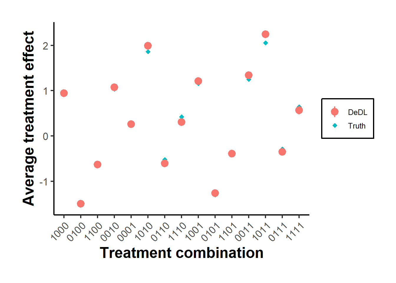
Figure 42.1: DeDL point estimates and 95 percent confidence intervals against ground truth for every treatment combination in the synthetic replication. Combinations marked as observed were part of the training support; the rest were never seen during training.
The DeDL confidence intervals cover the true effect for essentially every combination, including those the network never saw a single training example of, which is the payoff of Neyman orthogonality: the debiasing term corrects for the network’s residual approximation error well enough to deliver valid inference on combinations entirely outside the training support.
42.4.7 The Cost of Linear Additivity as Experiments Scale Up
The platform’s central practical question is how badly the default linear-addition heuristic degrades as more experiments run concurrently. We repeat the exercise above for \(m \in \{3,4,5\}\) concurrent experiments, each replicated twice with independently redrawn nuisance functions to average out simulation noise, exactly the design of the paper’s own Section 5.1 robustness check.
run_dedl_experiment <- function(m, dX = 10L, n_epochs = 400L, seed = 1) {
  set.seed(seed); torch_manual_seed(seed)

  A <- matrix(runif((m + 1) * dX, -0.5, 0.5), nrow = m + 1)
  theta_m1_true <- runif(1, 10, 20)
  theta_star <- function(X) { raw <- X %*% t(A); sign(raw) * abs(raw)^3 }
  G_true <- function(X, Tmat) {
    th <- theta_star(X)
    u <- th[, 1] + rowSums(th[, -1, drop = FALSE] * Tmat)
    theta_m1_true / (1 + exp(-u))
  }

  all_combos <- as.matrix(expand.grid(rep(list(0:1), m)))
  obs_support <- all_combos[rowSums(all_combos) %in% c(0, 1), , drop = FALSE]
  extra <- rep(0, m); extra[1:2] <- 1
  obs_support <- rbind(obs_support, extra)
  storage.mode(obs_support) <- "double"
  n_support <- nrow(obs_support)
  t0 <- rep(0, m)

  sample_partial <- function(n) {
    X <- matrix(runif(n * dX), n, dX)
    idx <- sample.int(n_support, n, replace = TRUE)
    Tmat <- obs_support[idx, , drop = FALSE]
    y <- G_true(X, Tmat) + runif(n, -0.05, 0.05)
    list(X = X, T = Tmat, y = y)
  }

  train <- sample_partial(500L * m)

  net <- nn_module(
    initialize = function(dX, hidden, out_dim) {
      self$fc1 <- nn_linear(dX, hidden)
      self$fc2 <- nn_linear(hidden, hidden)
      self$fc3 <- nn_linear(hidden, out_dim)
    },
    forward = function(x) x |> self$fc1() |> nnf_relu() |> self$fc2() |> nnf_relu() |> self$fc3()
  )
  model <- net(dX, hidden = 10L, out_dim = m + 1L)
  theta_m1_hat <- torch_tensor(15, requires_grad = TRUE)

  Xtr <- torch_tensor(train$X, dtype = torch_float())
  Ttr <- torch_tensor(train$T, dtype = torch_float())
  ytr <- torch_tensor(train$y, dtype = torch_float())
  opt <- optim_adam(c(model$parameters, list(theta_m1_hat)), lr = 0.01)

  forward_G <- function(X, Tt) {
    th <- model(X)
    u <- th[, 1] + torch_sum(th[, 2:(m + 1)] * Tt, dim = 2)
    theta_m1_hat / (1 + torch_exp(-u))
  }
  for (epoch in seq_len(n_epochs)) {
    opt$zero_grad()
    loss <- nnf_mse_loss(forward_G(Xtr, Ttr), ytr)
    loss$backward(); opt$step()
  }

  theta_hat_fn <- function(X) {
    with_no_grad({ th <- model(torch_tensor(X, dtype = torch_float())) })
    as.matrix(th)
  }
  theta_m1_val <- as.numeric(theta_m1_hat)

  G_hat_row <- function(th_row, t) theta_m1_val / (1 + exp(-(th_row[1] + sum(th_row[-1] * t))))
  Gtheta_hat_row <- function(th_row, t) {
    u <- th_row[1] + sum(th_row[-1] * t)
    s <- 1 / (1 + exp(-u)); ds <- s * (1 - s)
    c(theta_m1_val * ds, theta_m1_val * ds * t, s)
  }

  inf_data <- sample_partial(500L * m)
  th_inf <- theta_hat_fn(inf_data$X)
  d <- m + 2L
  n_inf <- nrow(inf_data$X)

  correction <- matrix(0, n_inf, d)
  for (i in seq_len(n_inf)) {
    th_i <- th_inf[i, ]
    Lam <- matrix(0, d, d)
    for (k in seq_len(n_support)) {
      g <- Gtheta_hat_row(th_i, obs_support[k, ])
      Lam <- Lam + outer(g, g)
    }
    Lam <- Lam * 2 / n_support + diag(0.0005, d)
    g_ti <- Gtheta_hat_row(th_i, inf_data$T[i, ])
    ell_th <- 2 * g_ti * (G_hat_row(th_i, inf_data$T[i, ]) - inf_data$y[i])
    correction[i, ] <- solve(Lam, ell_th)
  }

  lr_dat <- data.frame(y = train$y, train$X, train$T)
  names(lr_dat) <- c("y", paste0("x", seq_len(dX)), paste0("t", seq_len(m)))
  lr_fit <- lm(y ~ ., data = lr_dat)

  y0 <- mean(train$y[rowSums(train$T) == 0])
  la_effects <- sapply(seq_len(m), function(k) {
    sel <- train$T[, k] == 1 & rowSums(train$T) == 1
    mean(train$y[sel]) - y0
  })

  Xmc <- matrix(runif(10000L * dX), 10000L, dX)
  mu_true <- function(t) mean(G_true(Xmc, matrix(t, nrow(Xmc), m, byrow = TRUE))) -
                          mean(G_true(Xmc, matrix(t0, nrow(Xmc), m, byrow = TRUE)))

  out <- data.frame()
  for (k in seq_len(nrow(all_combos))) {
    t_target <- as.numeric(all_combos[k, ])
    if (all(t_target == t0)) next
    truth <- mu_true(t_target)

    Hx  <- sapply(seq_len(n_inf), function(i) G_hat_row(th_inf[i, ], t_target) - G_hat_row(th_inf[i, ], t0))
    Hth <- t(sapply(seq_len(n_inf), function(i) Gtheta_hat_row(th_inf[i, ], t_target) - Gtheta_hat_row(th_inf[i, ], t0)))
    psi <- Hx - rowSums(Hth * correction)

    newx  <- data.frame(matrix(runif(2000L * dX), 2000L, dX)); names(newx) <- paste0("x", seq_len(dX))
    newt1 <- as.data.frame(matrix(t_target, 2000L, m, byrow = TRUE)); names(newt1) <- paste0("t", seq_len(m))
    newt0 <- as.data.frame(matrix(t0, 2000L, m, byrow = TRUE)); names(newt0) <- paste0("t", seq_len(m))

    out <- rbind(out, data.frame(
      m = m, truth = truth,
      LA = sum(la_effects[t_target == 1]),
      LR = mean(predict(lr_fit, cbind(newx, newt1))) - mean(predict(lr_fit, cbind(newx, newt0))),
      SDL = mean(Hx), DeDL = mean(psi)
    ))
  }
  rm(model, opt, Xtr, Ttr, ytr, th_inf, correction)
  out
}

# Two replicates per m keep the sweep's total runtime bounded; gc() after each
# replicate prevents torch's per-call tensor allocations from accumulating
# across the loop, which otherwise slows later iterations substantially.
sweep_results <- data.frame()
for (m_val in c(3L, 4L, 5L)) {
  for (rep in 1:2) {
    r <- run_dedl_experiment(m_val, n_epochs = 300L, seed = 100 * m_val + rep)
    sweep_results <- rbind(sweep_results, r)
    gc(full = TRUE)
  }
}

mae_by_m <- aggregate(
  cbind(LA = abs(LA - truth), LR = abs(LR - truth), SDL = abs(SDL - truth), DeDL = abs(DeDL - truth)) ~ m,
  data = sweep_results, FUN = mean
)
mae_long <- reshape(mae_by_m, direction = "long", varying = c("LA", "LR", "SDL", "DeDL"),
                     v.names = "MAE", timevar = "Estimator", times = c("LA", "LR", "SDL", "DeDL"))

ggplot(mae_long, aes(x = m, y = MAE, color = Estimator)) +
  geom_line() +
  geom_point() +
  labs(x = "Number of concurrent experiments (m)", y = "Mean absolute error vs. ground truth") +
  causalverse::ama_theme()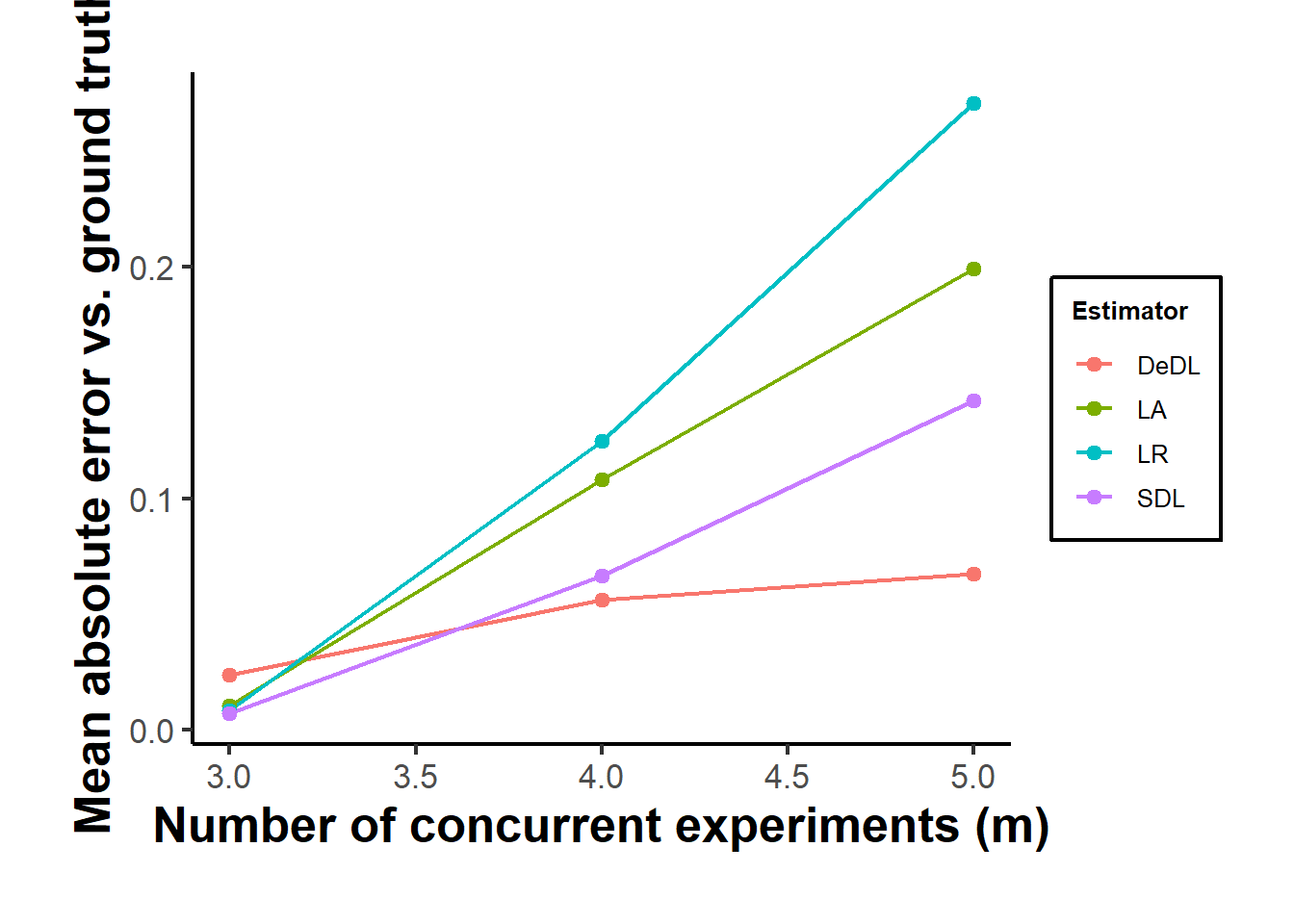
Figure 42.2: Mean absolute error against ground truth as the number of concurrent experiments m increases, averaged over two independently redrawn synthetic environments per m. The linear-addition and linear-regression benchmarks assume additive effects and degrade as more experiments interact; the structured deep network, with or without debiasing, uses the same \(m+2\) observed combinations regardless of m and remains comparatively stable.
The qualitative pattern matches the paper’s own Figure 8: the linear-addition and linear-regression estimators, which hard-code an additive structure that becomes more wrong as more experiments interact, do not improve as \(m\) grows and often worsen, while the structured network, trained on only \(m+2\) observed combinations no matter how large \(m\) is, holds up because its sigmoid link nests genuine nonlinear interaction. This is the practical case for the framework: a platform that already runs hundreds of concurrent experiments cannot expand its factorial coverage as \(m\) grows, but a structured, orthogonalized deep network can still deliver valid, increasingly necessary estimates of combinations it has never tested.
42.4.8 Practical Guidance
Three lessons from Ye et al. (2025) are worth carrying forward whenever deep learning is combined with Neyman orthogonality on a structural model layer rather than an unrestricted regression. First, the debiasing term is only as good as the first-stage network; when training has not converged, plain plug-in and debiased estimates are similar, and the value of debiasing appears only once training loss is genuinely small, so cross-validation loss during training is a useful diagnostic before trusting the debiased estimate. Second, a misspecified link function is more dangerous with debiasing than without, because the correction term amplifies rather than removes bias from a structural form that does not nest the truth; comparing the structured network’s validation loss against an unrestricted “pure DNN” that takes treatment as a raw input alongside the covariates, exactly the PDL benchmark Ye et al. (2025) use in Table 3, is a practical specification check that does not require knowing the true link function in advance. Third, and most important for scale, the framework’s traffic requirement grows linearly rather than exponentially in the number of concurrent experiments, which is what turns a theoretically elegant debiasing result into something a platform running hundreds of A/B tests can actually deploy.
42.5 Heterogeneous Treatment Effects
Average effects answer whether a treatment works on the whole. Many questions instead concern for whom it works, which is captured by the conditional average treatment effect (CATE) \[ \tau(x) = \mathbb{E}\bigl[Y(1) - Y(0) \mid X = x\bigr]. \] Estimating \(\tau(x)\) is a function-estimation problem rather than a scalar-estimation problem, and it is where tree-based and meta-learning methods come into their own.
42.5.1 Causal Forests and Generalized Random Forests
Causal forests, introduced by Wager and Athey (2018), adapt the random forest to estimate \(\tau(x)\) rather than a conditional mean. The key conceptual move, developed more generally in the generalized random forest of Athey et al. (2019), is to view a forest not as an ensemble of predictions but as an adaptive kernel or weighting function. A forest grown on the data assigns to a target point \(x\) a set of similarity weights \(\alpha_i(x)\), the frequency with which training observation \(i\) falls in the same leaf as \(x\) across the trees, \[ \alpha_i(x) = \frac{1}{B}\sum_{b=1}^{B} \frac{\mathbf{1}\{X_i \in L_b(x)\}}{\lvert L_b(x)\rvert}, \] where \(L_b(x)\) is the leaf of tree \(b\) containing \(x\). These weights then define a local, weighted version of any estimating equation. For heterogeneous effects the local estimating equation is a residualized treatment-effect regression, in the spirit of the R-learner described below, so the forest solves a weighted partialling-out problem in the neighborhood of each \(x\). This connects causal forests directly to the orthogonalization theme of the chapter.
Two features make the inference valid. First, the trees split to maximize heterogeneity in the treatment effect rather than to predict the outcome, so the adaptive neighborhoods are tailored to the causal target. Second, the forest uses honest splitting: the sample used to choose the splits is disjoint from the sample used to estimate the effect within each leaf. Honesty removes the overfitting bias that adaptive partitioning would otherwise introduce and is what allows Wager and Athey (2018) to derive asymptotic normality of the pointwise estimates, hence pointwise confidence intervals for \(\tau(x)\). The generalized random forest of Athey et al. (2019) extends the same kernel-weighting and honesty principles to a broad class of moment-condition problems, including instrumental variables and quantile estimation, and provides the theoretical foundation in the Annals of Statistics. An accessible empirical walkthrough appears in Athey and Wager (2019).
The following simulation builds the honest-forest CATE estimate conceptually using only base R, generating heterogeneous effects driven by a single covariate.
set.seed(2024)
n <- 4000
p <- 5
X <- matrix(runif(n * p), n, p)
e <- 0.5                                   # randomized treatment for clarity
W <- rbinom(n, 1, e)
tau_fun <- function(x) 1 + 2 * (x[, 1] > 0.5)   # effect doubles past 0.5
mu0 <- function(x) x[, 2] + sin(2 * pi * x[, 3])
Y <- mu0(X) + W * tau_fun(X) + rnorm(n)

# Stratified difference-in-means as a transparent CATE proxy:
# compare treated vs control within bins of the effect modifier X1.
bins <- cut(X[, 1], breaks = seq(0, 1, by = 0.25), include.lowest = TRUE)
cate_by_bin <- tapply(seq_len(n), bins, function(idx) {
    mean(Y[idx][W[idx] == 1]) - mean(Y[idx][W[idx] == 0])
})
round(cate_by_bin, 2)
#>   [0,0.25] (0.25,0.5] (0.5,0.75]   (0.75,1]
#>       1.06       1.08       3.06       3.09
The estimated effect jumps as \(X_1\) crosses 0.5, recovering the simulated heterogeneity. A causal forest automates this binning adaptively and over many covariates at once. The production estimator uses the grf package.
library(grf)

cf <- causal_forest(
    X = X, Y = Y, W = W,
    num.trees = 2000,
    honesty = TRUE
)

# Out-of-bag CATE predictions and pointwise standard errors
tau_hat <- predict(cf, estimate.variance = TRUE)
head(tau_hat)

# Doubly robust average treatment effect from the forest
average_treatment_effect(cf)

# Test for the presence of heterogeneity
test_calibration(cf)
42.5.2 The R-Learner and Meta-Learners
A complementary, modular philosophy estimates the CATE by reducing it to a sequence of standard prediction problems, each of which can be solved with any off-the-shelf learner. These are the meta-learners. The S-learner trains a single model on the pooled data with treatment as an additional feature, then takes the difference in predictions setting \(W = 1\) versus \(W = 0\). The T-learner trains two separate outcome models, one per treatment arm, and differences them. The X-learner, proposed by Künzel et al. (2019), refines the T-learner by imputing individual treatment effects, regressing them on covariates within each arm, and combining the two CATE estimates with propensity-based weights. The X-learner performs especially well when the treatment groups are very unequal in size or when one potential-outcome surface is much smoother than the other, settings where the T-learner wastes data.
The R-learner formalizes the residualization idea as a loss function. Starting from the Robinson decomposition, one residualizes the outcome and the treatment on the covariates, \(\tilde{Y} = Y - \hat{m}(X)\) and \(\tilde{W} = W - \hat{e}(X)\), and then estimates the CATE by minimizing the weighted criterion \[ \hat{\tau}(\cdot) = \arg\min_{\tau}\; \frac{1}{n}\sum_{i=1}^{n}\Bigl(\tilde{Y}_i - \tau(X_i)\,\tilde{W}_i\Bigr)^2 + \Lambda\bigl(\tau\bigr), \] where \(\Lambda\) is a regularizer on the CATE function. Because the nuisances enter only through the residuals, the objective is Neyman orthogonal, so errors in \(\hat{m}\) and \(\hat{e}\) have a second-order effect on the estimated heterogeneity. Causal forests can be seen as solving a local version of this same R-learner objective, which is why the two approaches are tightly linked.
library(rlearner)   # R-, S-, T-, X-learners with glmnet or boosting

# R-learner with cross-validated lasso nuisances
rfit <- rlasso(x = X, w = W, y = Y)
tau_rlearner <- predict(rfit, X)

# X-learner via the same package family
xfit <- xboost(x = X, w = W, y = Y)
tau_xlearner <- predict(xfit, X)
The choice among meta-learners and forests is empirical. Forests provide honest pointwise inference and require little tuning; meta-learners offer flexibility in the choice of base learner and can exploit structure such as smoothness or sparsity. A common workflow estimates the CATE several ways and checks that the qualitative conclusions about who benefits are stable across methods.
42.6 Publishing With These Methods: A Marketing Targeting Study
The methods in this chapter are not only academically interesting; they are the engine behind a recognizable genre of empirical paper that publishes regularly in the top marketing and quantitative-marketing journals. Knowing the shape of that genre is useful both for reading the literature and for producing work that can survive its review process, so this section first describes the template and then replicates it end to end on a public dataset with production-grade code.
42.6.1 What a Publishable Paper Looks Like
The papers that use heterogeneous-treatment-effect machinery to publish in Marketing Science, the Journal of Marketing Research, Management Science, and Quantitative Marketing and Economics share a common skeleton, and the contribution is rarely the estimator itself, which is taken off the shelf, but the design and the decision it informs. The canonical reference is Hitsch et al. (2024), who lay out the modern recipe explicitly: start from a randomized experiment or a credibly exogenous source of variation that identifies the treatment effect without functional-form heroics, estimate the conditional average treatment effect with a causal forest, and then, crucially, evaluate targeting policies rather than reporting the CATE as an end in itself. Their central methodological insight, which separates a publishable paper from a classroom exercise, is that the quantity a manager cares about is the value of a policy that assigns treatment based on covariates, and that this policy value can be estimated with a doubly robust score even when the underlying CATE estimates are noisy. The estimand is the profit or outcome of a targeting rule, not the accuracy of the effect surface.
The substantive surprises that make such papers worth publishing usually come from the gap between the effect of a treatment and the characteristics that managers intuitively target. Ascarza (2018) provides the discipline’s clearest cautionary result, showing through field experiments that the customers at highest risk of churning, the natural target of a retention campaign, are not the customers whose behavior responds most to intervention, so that a campaign aimed at high-risk customers can be nearly worthless while the same budget aimed at high-responsiveness customers pays off. The lesson, that one should target the treatment effect rather than the baseline level, is exactly what a causal forest operationalizes, and it recurs across the literature. Simester et al. (2020) stress-test the machine-learning targeting pipeline against the data problems that real firms face, missing covariates, distribution shift between the experiment and the deployment population, and small samples, and document which methods degrade gracefully, a robustness contribution that is itself publishable. Yoganarasimhan et al. (2023) use these tools to design and evaluate optimal free-trial lengths for a subscription product, turning an estimated heterogeneous effect into a personalized policy and quantifying its lift over the firm’s status quo, while Rafieian and Yoganarasimhan (2021) bring the same logic to mobile advertising and weigh the targeting gains against their privacy costs.
A second strand earns its place by getting the identification right at scale rather than by the heterogeneity machinery. Gordon et al. (2019) compare experimental and observational advertising-effect estimates across large Facebook field experiments and show how far selection-on-observables adjustments, including propensity and double-machine-learning style methods, fall short of the experimental benchmark, a sobering result about the limits of observational causal inference in marketing. Dube and Misra (2023) run experiments to estimate personalized price elasticities and then compute the welfare consequences of personalized pricing, combining experimentation, heterogeneous-effect estimation, and a welfare calculation into one paper. On the methodological side, Knaus et al. (2021) give the kind of careful empirical Monte Carlo comparison of heterogeneous-effect estimators that lets applied researchers choose among causal forests, the R-learner, and the various meta-learners with evidence rather than fashion. The throughline is that the estimator is a commodity and the contribution lives in the design, the data, the policy question, and the honesty of the evaluation.
42.6.2 Replicating the Targeting Workflow on the Hillstrom Email Experiment
To make the recipe concrete we replicate its core on a genuinely public marketing field experiment, the email campaign released by Kevin Hillstrom through the MineThatData challenge, which has become a standard benchmark for targeting research because it is a real randomized experiment with customer covariates and behavioral outcomes. Sixty-four thousand customers were randomly assigned to receive an email featuring men’s merchandise, an email featuring women’s merchandise, or no email, and the data record whether each customer visited the site, made a purchase, and how much they spent in the following two weeks. We use the clean two-arm comparison of the women’s email against no email, with website visits as the outcome, and ask the question a manager actually faces: given the covariates, whom should we email?
email <- read.csv("data/hillstrom_email.csv")

# Clean two-arm experiment: women's email versus no email.
email <- email[email$segment %in% c("Womens E-Mail", "No E-Mail"), ]

W <- as.integer(email$segment == "Womens E-Mail")   # treatment: received email
Y <- email$visit                                     # outcome: visited the site

# Covariates the firm knows before sending: purchase recency, dollar history,
# past category, tenure, acquisition channel, and location type.
X <- data.frame(
  recency   = email$recency,
  history   = email$history,
  mens      = email$mens,
  womens    = email$womens,
  newbie    = email$newbie,
  phone     = as.integer(email$channel == "Phone"),
  web       = as.integer(email$channel == "Web"),
  zip_urban = as.integer(email$zip_code == "Urban"),
  zip_rural = as.integer(email$zip_code == "Rural")
)

c(customers = nrow(X), treated = sum(W), baseline_visit_rate = round(mean(Y), 4))
#>           customers             treated baseline_visit_rate
#>          42693.0000          21387.0000              0.1288
The first step is the credibility anchor, the average treatment effect. Because assignment was randomized, even a simple difference in means identifies it, but we estimate it from a causal forest so that the same fitted object delivers both the average effect and the heterogeneity. The forest residualizes the outcome and the treatment on the covariates internally, the orthogonalization of the earlier sections, and returns a doubly robust average effect.
library(grf)

set.seed(42)
cf <- causal_forest(as.matrix(X), Y, W, num.trees = 1000, seed = 42)

ate <- average_treatment_effect(cf, target.sample = "all")
calib <- test_calibration(cf)
tau_hat <- predict(cf)$predictions| Quantity | Estimate | Std. Error |
|---|---|---|
| Average treatment effect (visit prob.) | 0.0439 | 0.0033 |
| Heterogeneity test (differential.forest.prediction) | 0.4120 | 0.0700 |
The women’s email raises the probability of a site visit by roughly four percentage points off a baseline near thirteen percent, a large and precisely estimated effect. The calibration test of Wager and Athey (2018) regresses the held-out outcome on the mean forest prediction and on the demeaned forest prediction; the coefficient on the differential prediction is well above zero and many standard errors from it, which is the formal evidence that the effect genuinely varies across customers rather than the forest manufacturing spurious variation. Figure 42.3 shows the spread of the individual effect estimates, which range from slightly negative to well above the average, the raw material of any targeting decision.
library(ggplot2)

ggplot(data.frame(tau = tau_hat), aes(tau)) +
  geom_histogram(bins = 40) +
  geom_vline(xintercept = ate[["estimate"]], linetype = "dashed") +
  labs(x = "Estimated treatment effect on visit probability",
       y = "Number of customers") +
  causalverse::ama_theme()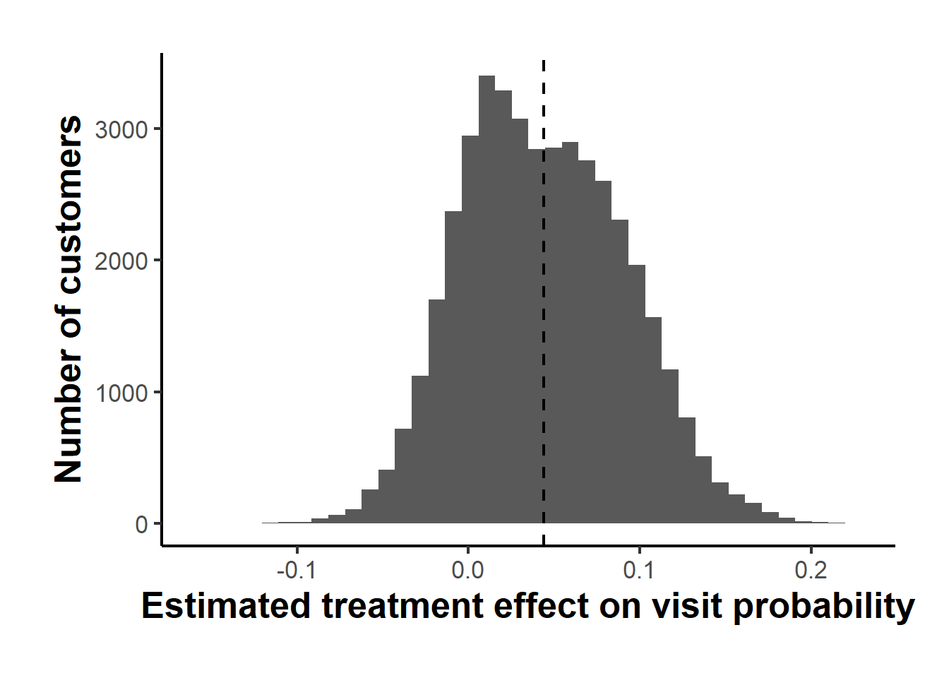
Figure 42.3: Distribution of estimated conditional average treatment effects of the women’s email on site visits across customers. The dashed line marks the average effect. A minority of customers have near-zero or negative estimated effects and are candidates for suppression.
Detecting heterogeneity is not the same as profiting from it, and the next step is the one Hitsch et al. (2024) insist on: quantify how much value a targeting rule that prioritizes by estimated effect actually delivers. The rank-weighted average treatment effect, computed by rank_average_treatment_effect, measures exactly this. It traces the average effect among the customers the model ranks most responsive as we expand the targeted fraction from the few down to everyone, and the area under that curve, the AUTOC, summarizes the gain from prioritizing by the estimated CATE over treating a random customer. Figure 42.4 plots the curve.
rate <- rank_average_treatment_effect(cf, tau_hat)

ggplot(rate$TOC, aes(q, estimate)) +
  geom_line() +
  geom_hline(yintercept = 0, linetype = "dotted") +
  labs(x = "Fraction of customers targeted (most responsive first)",
       y = "Average effect among targeted") +
  causalverse::ama_theme()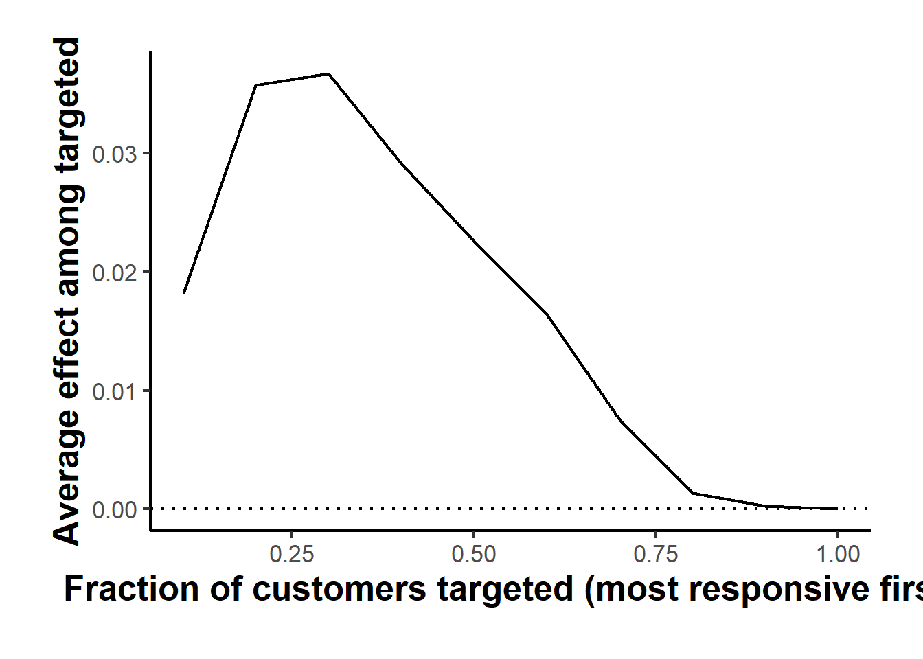
Figure 42.4: Targeting operator characteristic curve. The vertical axis is the average treatment effect among the top fraction of customers ranked by estimated responsiveness; the horizontal axis is that fraction. A curve lying above zero and sloping down means the model concentrates the effect in the customers it prioritizes, which is the value of targeting.
#> RATE (AUTOC): 0.0176 (std. error 0.0039)The curve slopes downward and the AUTOC is several standard errors above zero, so the forest is genuinely separating responsive from unresponsive customers rather than ranking them at random. The final step converts that ranking into a deployable rule and evaluates it honestly. The policytree package of Athey et al. (2019) learns a shallow, interpretable decision tree that maps covariates directly to a treat-or-not recommendation, fit on the doubly robust scores from the forest so that the learned policy inherits the orthogonality that protects it from nuisance error. We fit a depth-two tree on a subsample for speed and then evaluate several policies against the same doubly robust scores.
library(policytree)

dr_scores <- double_robust_scores(cf)

# Learn an interpretable depth-2 targeting rule (subsample for tractable search).
set.seed(7)
sub <- sample(nrow(X), 10000)
ptree <- policy_tree(X[sub, ], dr_scores[sub, ], depth = 2)

# Apply the rule to everyone; action 2 = send email, 1 = withhold.
send <- predict(ptree, X) == 2

# Doubly robust value of each policy: expected incremental visits per customer
# relative to emailing no one.
policy_value <- function(treat) mean(ifelse(treat, dr_scores[, 2], dr_scores[, 1]) - dr_scores[, 1])

value_table <- data.frame(
  Policy = c("Email no one", "Email everyone",
             "Email if estimated effect > 0", "Learned policy tree"),
  `Share emailed` = c(0, 1, mean(tau_hat > 0), mean(send)),
  `Incremental visits per customer` = c(
    0, policy_value(rep(TRUE, nrow(X))),
    policy_value(tau_hat > 0), policy_value(send)),
  check.names = FALSE
)| Policy | Share emailed | Incremental visits per customer |
|---|---|---|
| Email no one | 0.000 | 0.0000 |
| Email everyone | 1.000 | 0.0439 |
| Email if estimated effect > 0 | 0.814 | 0.0366 |
| Learned policy tree | 0.692 | 0.0420 |
The policy comparison is where the managerial payoff appears, and it carries the same counterintuitive flavor as Ascarza (2018). Because the email helps the great majority of customers, emailing everyone produces the largest raw lift in visits, and a naive reading would stop there. The learned policy tree, however, achieves nearly the same incremental visits while emailing only about seventy percent of the customers, which means the firm can shed roughly a third of its mailing cost for a small fraction of the benefit, and the tree is fully transparent about who it drops, splitting on past purchase history and category in a way a manager can inspect and defend. When the outcome is replaced by profit net of contact cost, as it would be in a deployment, the policies that look tied on raw visits separate sharply, and the targeting rule dominates the blanket campaign. This is precisely the structure of the published papers: a randomized design for identification, a flexible forest for the heterogeneity, an honest doubly robust evaluation of the policy rather than the effect, and a managerial conclusion that the obvious blanket strategy leaves money on the table.
The replication is also a template a reader can extend toward a publishable contribution. Swapping the visit outcome for spend turns the analysis into a revenue-targeting problem; subtracting a per-email cost converts the policy value into profit and sharpens the case for selective mailing; using all three experimental arms moves from a binary treatment to a multi-armed targeting problem that policytree handles directly; and validating the learned policy on a held-out portion of the experiment, or on the men’s-email arm, supplies the out-of-sample evidence that referees expect. The full toolchain, grf for the forest, rank_average_treatment_effect for the targeting value, and policytree for the deployable rule, is the same one behind the papers cited above, which is why working through it on public data is the most direct way to learn how such studies are built.
42.7 Temporal Causal Forests
The forest machinery extends naturally to settings with a strong temporal structure, where every unit is eventually exposed to a widely known event and a clean contemporaneous control group does not exist. This arises with public announcements, recalls, security breaches, and similar shocks, where it is impossible to find a group unaware of the event that would still be representative of the affected population. The temporal causal inference design of Turjeman and Feinberg (2023) addresses this by matching across cohorts that adopted at different times, so that newer participants who experienced the event early in their tenure are compared with the early trajectories of older participants who had not yet been exposed.
The core idea is to make calendar time and tenure separate axes. Let \(H_T\) denote the cohort that joined \(T\) time units before the event; this treated cohort is observed for \(T + 3\) units, with the final units after the event. Control trajectories are assembled from earlier cohorts \(H_1, \dots, H_{T-1}\), tracked from their own adoption up to the event or to the matched tenure window, whichever comes first. Each cohort plays a dual role, sometimes treated and sometimes control, except for those at the extreme ends of the window. Because the design relies on comparing trajectories rather than a single contemporaneous control, it requires a large sample so that subgroups with comparable time trends can be matched.
The figure below illustrates the design with simulated cohorts, showing the same activity curves on a calendar-time axis and on a tenure axis. On the tenure axis the cohorts line up, making clear that the control cohorts simply had not yet reached the event when the treated cohort did.
library(ggplot2)
library(patchwork)

tenure <- seq(0, 100, length.out = 100)
generate_cohort <- function(name, start_time, mean, sd) {
    data.frame(
        tenure = tenure,
        cohort = name,
        time   = seq(start_time, start_time + 99, by = 1),
        value  = dnorm(tenure, mean = mean, sd = sd)
    )
}
cohorts <- list(
    generate_cohort("Cohort 1",  1, 47, 15),
    generate_cohort("Cohort 2", 10, 48, 17),
    generate_cohort("Cohort 3", 20, 52, 20),
    generate_cohort("Cohort 4", 30, 53, 18),
    generate_cohort("treatment", 40, 50, 16)
)
final_dataset <- do.call(rbind, cohorts)

plot_time <- ggplot(final_dataset, aes(time, value, color = cohort)) +
    geom_line() +
    geom_vline(xintercept = c(40, 90), linetype = "dashed") +
    labs(title = "Value vs. Calendar Time", x = "Time", y = "Value")

plot_tenure <- ggplot(final_dataset, aes(tenure, value, color = cohort)) +
    geom_line() +
    geom_vline(xintercept = c(0, 50), linetype = "dashed") +
    labs(title = "Value vs. Tenure", x = "Tenure", y = "Value")

plot_time / plot_tenure
Identification rests on the usual selection-on-observables assumptions, reinterpreted for the temporal setting. The stable unit treatment value assumption requires no interference, which holds across cohorts because their treatment exposures occur at different points in calendar time, though it can be strained when treated units influence one another after the shock. Conditional independence requires that, given the covariates including the time trend, cohort membership is as good as randomly assigned; this is checked empirically with pre-treatment parallel-trends tests, including bidirectional Granger tests and Kolmogorov-Smirnov comparisons of the pre-event trajectories. Overlap requires that every unit had a positive propensity of treatment at any tenure, which the design satisfies because all units are eventually treated and the estimated propensity is bounded away from zero and one. Exogeneity of covariates requires that the shock was unforeseen, or at least equally anticipated across cohorts.
Temporal causal forests then extend the causal forest in two ways identified by Turjeman and Feinberg (2023) as improving root-mean-squared error and recovery of heterogeneous effects. First, the covariate vector \(X_i\) is augmented to include the unit’s time trend, so the forest groups units that are homogeneous in their activity trajectories, in effect estimating a counterfactual time path for each unit and ensuring that treated and control units share similar pre-event trends. Second, as a robustness analysis, the nuisance functions are estimated with the local linear forest of Friedberg et al. (2020), which fits a local linear correction within each leaf and improves accuracy when the underlying surface is smooth; this refinement is feasible when cohort timelines are of equal length. The result is a method that recovers both the average effect of a public shock and its heterogeneity across individuals while respecting the temporal structure that rules out a conventional control group.
42.8 Practical Guidance and Pitfalls
Several practical considerations govern whether these methods deliver on their promise.
Cross-fitting is not optional. The asymptotic guarantees of double machine learning depend on estimating the nuisance functions on data separate from the data used to form the final estimate. Skipping this step reintroduces overfitting bias and invalidates the confidence intervals, even when an orthogonal score is used.
Orthogonality protects only against slow nuisance errors, not against violations of identification. If unconfoundedness fails because an important confounder is unobserved, no amount of flexible nuisance estimation will recover the causal effect. Machine learning strengthens the case for conditional ignorability by allowing a rich conditioning set, but it cannot test the assumption itself. The role of these methods is to remove functional-form and high-dimensionality concerns, leaving the identifying assumptions to be defended on substantive grounds.
Overlap matters more, not less, with flexible models. Inverse propensity weights become unstable when estimated propensities approach zero or one, and flexible learners can produce extreme propensity estimates. Diagnosing the propensity distribution, trimming or stabilizing extreme weights, and preferring substitution estimators such as TMLE that are less sensitive to small denominators all help. Reporting the distribution of estimated propensity scores should be routine.
Heterogeneity claims require discipline. A causal forest will always produce a varying \(\tau(x)\), but the variation may be noise. The honest forest delivers pointwise standard errors, and calibration tests such as the best-linear-predictor test assess whether the estimated heterogeneity is real. Out-of-sample validation, for instance ranking units by predicted effect and checking that the realized effect ordering agrees, guards against overinterpreting spurious patterns.
Sample size and tuning are real constraints. Like other nonparametric and matching methods, forests and meta-learners need substantial data for stable results, especially when estimating heterogeneity across many covariates or when treatment groups are imbalanced. The SuperLearner reduces the burden of choosing a single learner, but it multiplies computation, and the analyst should ensure that the cross-validation used inside the ensemble is nested properly within the cross-fitting used for the causal estimate.
Finally, transparency and replication remain essential. The flexibility that makes these methods powerful also makes them harder to scrutinize. Pre-registering the estimand, the conditioning set, and the validation plan, and reporting results across several estimators, keeps the analysis honest and the conclusions credible.