35 Difference-in-Differences

Difference-in-Differences (DID) is a widely used causal inference method for estimating the effect of policy interventions or exogenous shocks when randomized experiments are not feasible. The key idea behind DID is to compare changes in outcomes over time between treated and control groups, under the assumption that, absent treatment, both groups would have followed parallel trends.

The method is well suited to business analytics because transaction logs, panel dashboards, and quarterly filings already furnish the required data. Its identifying assumptions are easy to communicate, and it controls for economy-wide shocks without heavy modeling.

Practical Advantages of DID

• Intuitive visuals: A two-line plot can immediately signal whether pre-treatment trends look parallel.
• Light data demands: Only two time points and a clear treatment onset are needed.
• Extendable: Regression frameworks accommodate staggered treatments, multiple periods, or continuous exposures.
• Transparent: Assumptions and identifying variation are easy to communicate to executives, regulators, or reviewers.

DID analysis can go beyond simple treatment effects by exploring causal mechanisms using mediation and moderation analyses:

• Mediation Under DiD: Examines how intermediate variables (e.g., consumer sentiment, brand perception) mediate the treatment effect (Habel et al. 2021).
• Moderation Analysis: Studies how treatment effects vary across different groups (e.g., high vs. low brand loyalty) (Goldfarb and Tucker 2011).

The remainder of this chapter develops DID estimation, diagnoses its assumptions, and shows how to defend findings against the standard concerns raised by reviewers and other audiences. The exposition leads with intuition and applied cases before introducing the corresponding formalism.

35.1 Where DID has been put to work

The published record of DID studies is enormous, but it is worth pausing on a handful of representative applications because the kinds of questions DID has answered tell you a great deal about the kinds of question it can answer well, namely, questions in which a sharp policy or competitive event hits one group while leaving a comparable group untouched, with the outcomes of both observable before and after.

In marketing and business, the canonical questions concern how consumers and firms respond to interventions that arrive as discrete events. Several studies trace the impact of advertising and content on consumer behaviour: Liaukonyte et al. (2015) show how TV ads ripple into online shopping, Wang et al. (2018) use geographic discontinuities at state borders to disentangle the effect of political ad source and tone on turnout, and Datta et al. (2018) track how adopting a music-streaming service reshapes total consumption. A second cluster studies how firms react to digital and regulatory shocks. Janakiraman et al. (2018) trace how customer spending shifts after a publicly announced data breach; Israeli (2018) ask whether digital monitoring tightens enforcement of minimum-advertised-price policies; Ramani and Srinivasan (2019) examine how Indian firms responded to the 1991 FDI liberalization; Pattabhiramaiah et al. (2019) quantify the readership cost of newspaper paywalls; Akca and Rao (2020) study how online aggregators reshape airline-ticket sales; Lim et al. (2020) ask whether nutritional labels nudge competing brands toward healthier formulations; Guo et al. (2020) examine how payment-disclosure laws reach into physician prescribing; He et al. (2022) exploit an Amazon policy change to measure the effect of fake reviews on sales and ratings; and Peukert et al. (2022) assess how GDPR rewired website usage and online business models. The common ingredient across all of these is a clean event date and a credible comparison group, without both, the design loses its bite.

DID has been at least as central in economics, where it underpins much of modern policy evaluation. Rosenzweig and Wolpin (2000)’s review of natural experiments in development economics maps the design’s reach in that subfield; Angrist and Krueger (2001) connect DID to instrumental-variable thinking by showing how natural experiments can serve both purposes; and Fuchs-Schündeln and Hassan (2016) extend the logic to macroeconomic policy analysis, where unit heterogeneity is severe and the parallel-trends assumption demands particular care.

---

35.2 Visualization

Before diving into estimation, it is always wise to (i) confirm the treatment pattern and (ii) eyeball the outcomes.

The panelView package offers quick heatmaps and outcome traces that make these checks straightforward.

35.2.1 Data check

library(panelView)
library(fixest)
library(tidyverse)
base_stagg <- fixest::base_stagg |>
    # treatment status
    dplyr::mutate(treat_stat = dplyr::if_else(time_to_treatment < 0, 0, 1)) |> 
    select(id, year, treat_stat, y)

head(base_stagg)
#>   id year treat_stat           y
#> 2 90    1          0  0.01722971
#> 3 89    1          0 -4.58084528
#> 4 88    1          0  2.73817174
#> 5 87    1          0 -0.65103066
#> 6 86    1          0 -5.33381664
#> 7 85    1          0  0.49562631

35.2.2 Treatment Assignment Heatmap

Figure 35.1 shows the heatmap of treatment status for each unit over 10 years.

panelView::panelview(
    y ~ treat_stat,
    data = base_stagg,
    index = c("id", "year"),
    xlab = "Year",
    ylab = "Unit",
    display.all = F,
    gridOff = T,
    by.timing = T
)

Figure 35.1: Treatment assignment over time by unit.

The diagonal “step” confirms that not all units adopt at once. This would be perfect for a staggered-DiD design. Horizontal segments without a color change indicate units that never adopt.

Alternatively, specifying the outcome and treatment status will also return the exact figure (Figure 35.2)

# alternatively specification
panelView::panelview(
    Y = "y",
    D = "treat_stat",
    data = base_stagg,
    index = c("id", "year"),
    xlab = "Year",
    ylab = "Unit",
    display.all = F,
    gridOff = T,
    by.timing = T
)

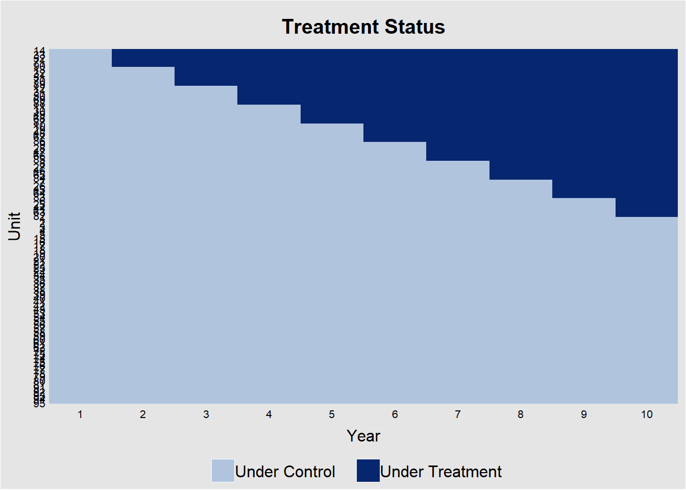
Figure 35.2: Staggered treatment timing across units.

35.2.3 Raw Outcome Trajectories

Figure 35.3 shows the trajectories of different cohorts over time.

# Average outcomes for each cohort
panelView::panelview(
    data = base_stagg, 
    Y = "y",
    D = "treat_stat",
    index = c("id", "year"),
    by.timing = T,
    display.all = F,
    type = "outcome", 
    by.cohort = T
)
#> Number of unique treatment histories: 10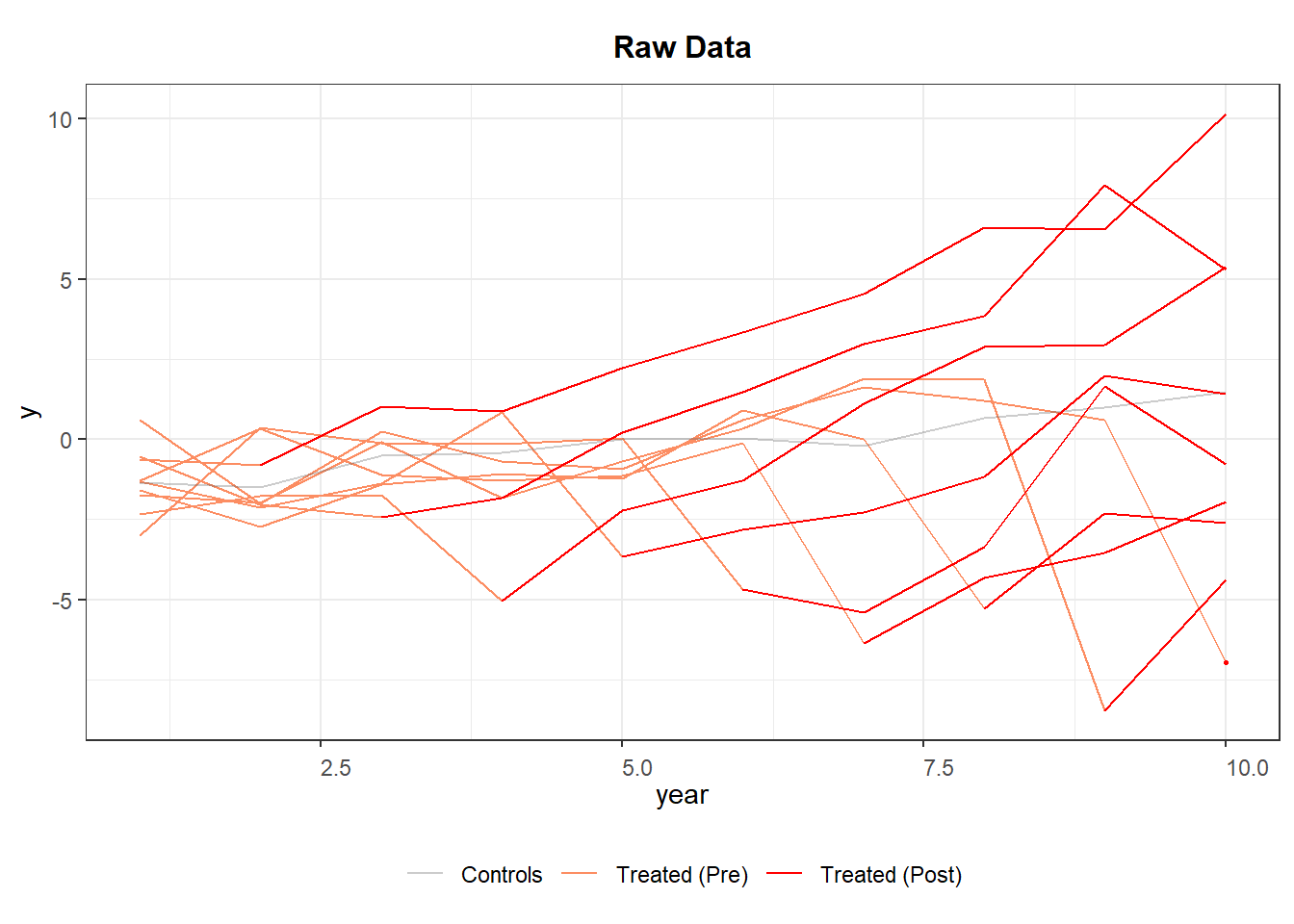

Figure 35.3: Raw panel data by treatment status over time.

If the red segments diverge immediately after treatment while the orange segments blend with gray beforehand, the visual evidence is supportive of a treatment effect and parallel pre-trends.

35.2.4 Event-time Averages

A more focused diagnostic is to plot the average outcome in event time (years relative to first treatment) (Figure 35.4).

base_stagg |>
    group_by(event_time = year - min(year[treat_stat == 1])) |>
    summarise(y_mean = mean(y),
              se     = sd(y) / sqrt(n())) |>
    ggplot(aes(event_time, y_mean)) +
    geom_line(color = "#377eb8", linewidth = 1) +
    geom_ribbon(aes(ymin = y_mean - se, ymax = y_mean + se),
                fill = "#377eb8",
                alpha = .2) +
    geom_vline(xintercept = 0, linetype = "dashed") +
    labs(x = "Years relative to treatment",
         y = "Mean outcome (y)",
         title = "Event-time plot: do outcomes change at treatment onset?") +
    theme_minimal()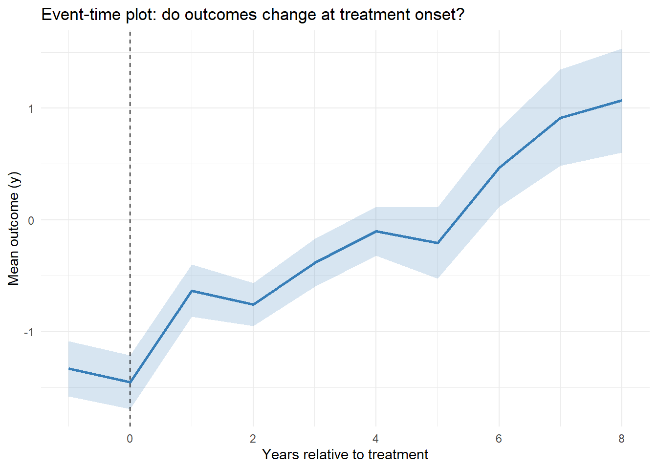

Figure 35.4: Event-time averages of the outcome relative to treatment onset.

A flat pre-trend (negative event times) and a noticeable jump at event-time 0 support the identifying assumptions for staggered DiD.

35.3 Simple Difference-in-Differences

DID first emerged as a tool for natural experiments, settings where policy shocks or geographic quirks mimic random assignment. Its scope has since broadened: marketing A/B roll-outs, corporate ESG mandates, and the staggered release of a mobile-app feature now routinely call on DID for credible impact estimates.

At its computational heart lies the Fixed Effects Estimator, which sweeps out any time-invariant heterogeneity across units and any shocks common to all periods, leaving the residual variation that identifies the treatment effect.

DID exploits inter-temporal variation between groups in two complementary ways to address omitted variable bias:

• Cross-sectional comparison: Compares treated and control units at the same point in time, canceling bias from shocks that hit both groups equally (e.g., nationwide inflation). This helps avoid omitted variable bias due to common trends.
• Time-series comparison: Tracks the same unit over time, purging bias from any fixed, unit-specific traits (e.g., a chain’s brand equity, a region’s climate). This helps mitigate omitted variable bias due to cross-sectional heterogeneity.

By taking the difference of differences, we simultaneously:

1. Remove common trends that could confound a simple cross-sectional comparison.
2. Eliminate unit-specific constants that would spoil a pure time-series analysis.

---

35.3.1 Basic Setup of DID

Consider a simple setting in Table 35.1 with:

• Treatment Group (\(D_i = 1\))
• Control Group (\(D_i = 0\))
• Pre-Treatment Period (\(T = 0\))
• Post-Treatment Period (\(T = 1\))

Table 35.1: Potential outcomes by treatment status and time.

	After Treatment (\(T = 1\))	Before Treatment (\(T = 0\))
Treated (\(D_i = 1\))	\(E[Y_{1i}(1)|D_i = 1]\)	\(E[Y_{0i}(0)|D_i = 1]\)
Control (\(D_i = 0\))	\(E[Y_{0i}(1)|D_i = 0]\)	\(E[Y_{0i}(0)|D_i = 0]\)

The fundamental challenge: We cannot observe \(E[Y_{0i}(1)|D_i = 1]\) (i.e., the counterfactual outcome for the treated group had they not received treatment).

---

DID estimates the Average Treatment Effect on the Treated using the following formula:

\[ \begin{aligned} E[Y_1(1) - Y_0(1) | D = 1] &= \{E[Y(1)|D = 1] - E[Y(1)|D = 0] \} \\ &- \{E[Y(0)|D = 1] - E[Y(0)|D = 0] \} \end{aligned} \]

What parallel trends really says. The identifying assumption is a statement about the untreated potential outcome of the treated group, an object we never observe post-treatment:

\[ E[Y(0)_{t=1} - Y(0)_{t=0} \mid D = 1] = E[Y(0)_{t=1} - Y(0)_{t=0} \mid D = 0]. \]

That is, had the treated group not been treated, its average outcome would have evolved in parallel with the control group’s. This is intrinsically counterfactual and therefore untestable in the post-treatment period.

What pre-trend plots and placebo tests check is whether the observed pre-treatment trends were parallel. A clean pre-trend is supportive evidence for, but not proof of, the identifying assumption. Roth (2022) shows that conventional pre-trend tests often have low power, so “failing to reject” is weak evidence at best. Modern practice couples pre-trend diagnostics with formal sensitivity analysis (e.g., Rambachan and Roth (2023); see Section 35.13).

This formulation differences out time-invariant unobserved factors, assuming the parallel trends assumption holds.

• For the treated group, we isolate the difference between being treated and not being treated.
• If the control group would have experienced a different trajectory, the DID estimate may be biased.
• Since we cannot observe treatment variation in the control group, we cannot infer the treatment effect for this group.

# Load required libraries
library(dplyr)
library(ggplot2)
set.seed(1)

# Simulated dataset for illustration
data <- data.frame(
  time = rep(c(0, 1), each = 50),  # Pre (0) and Post (1)
  treated = rep(c(0, 1), times = 50), # Control (0) and Treated (1)
  error = rnorm(100)
)

# Generate outcome variable
data$outcome <-
    5 + 3 * data$treated + 2 * data$time + 
    4 * data$treated * data$time + data$error

# Compute averages for 2x2 table
table_means <- data %>%
  group_by(treated, time) %>%
  summarize(mean_outcome = mean(outcome), .groups = "drop") %>%
  mutate(
    group = paste0(ifelse(treated == 1, "Treated", "Control"), ", ", 
                   ifelse(time == 1, "Post", "Pre"))
  )

# Display the 2x2 table
table_2x2 <- table_means %>%
  select(group, mean_outcome) %>%
  tidyr::spread(key = group, value = mean_outcome)

print("2x2 Table of Mean Outcomes:")
#> [1] "2x2 Table of Mean Outcomes:"
print(table_2x2)
#> # A tibble: 1 × 4
#>   `Control, Post` `Control, Pre` `Treated, Post` `Treated, Pre`
#>             <dbl>          <dbl>           <dbl>          <dbl>
#> 1            7.19           5.20            14.0           8.00

# Calculate Diff-in-Diff manually

# Treated, Post
Y11 <- table_means$mean_outcome[table_means$group == "Treated, Post"]  

# Treated, Pre
Y10 <- table_means$mean_outcome[table_means$group == "Treated, Pre"]   

# Control, Post
Y01 <- table_means$mean_outcome[table_means$group == "Control, Post"]  

# Control, Pre
Y00 <- table_means$mean_outcome[table_means$group == "Control, Pre"]   

diff_in_diff_formula <- (Y11 - Y10) - (Y01 - Y00)

# Estimate DID using OLS
model <- lm(outcome ~ treated * time, data = data)
ols_estimate <- coef(model)["treated:time"]

# Print results
results <- data.frame(
  Method = c("Diff-in-Diff Formula", "OLS Estimate"),
  Estimate = c(diff_in_diff_formula, ols_estimate)
)

print("Comparison of DID Estimates:")
#> [1] "Comparison of DID Estimates:"
print(results)
#>                            Method Estimate
#>              Diff-in-Diff Formula 4.035895
#> treated:time         OLS Estimate 4.035895

Figure 35.5 shows a simple visualization of the DID in practice.

# Visualization
ggplot(data,
       aes(
           x = as.factor(time),
           y = outcome,
           color = as.factor(treated),
           group = treated
       )) +
    stat_summary(fun = mean, geom = "point", size = 3) +
    stat_summary(fun = mean,
                 geom = "line",
                 linetype = "dashed") +
    labs(
        title = "Difference-in-Differences Visualization",
        x = "Time (0 = Pre, 1 = Post)",
        y = "Outcome",
        color = "Group"
    ) +
    scale_color_manual(labels = c("Control", "Treated"),
                       values = c("blue", "red")) +
    causalverse::ama_theme()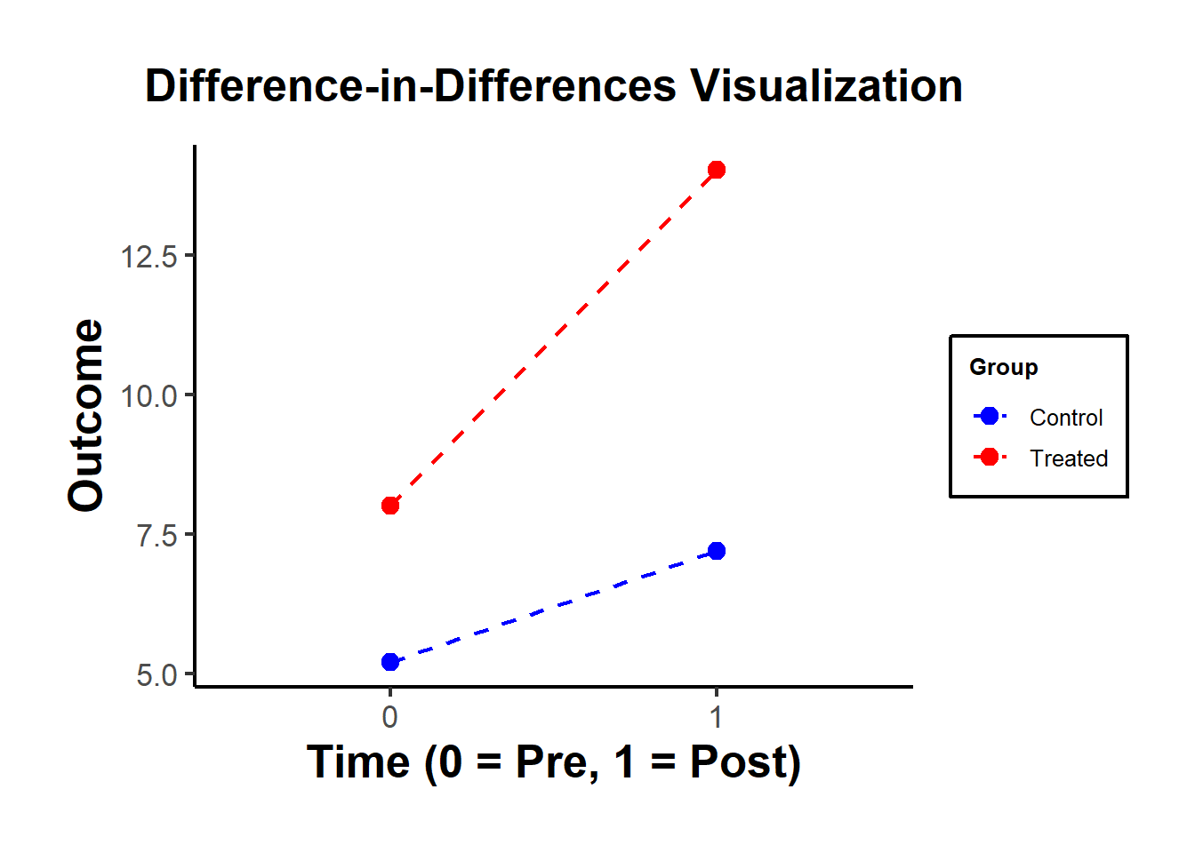

Figure 35.5: DiD visualization of treated and control group changes pre- and post-intervention.

Table 35.2: DiD table of group-time average outcomes.

	Control (0)	Treated (1)
Pre (0)	\(\bar{Y}_{00} = 5\)	\(\bar{Y}_{10} = 8\)
Post (1)	\(\bar{Y}_{01} = 7\)	\(\bar{Y}_{11} = 14\)

Table 35.2 organizes the mean outcomes into four cells:

1. Control Group, Pre-period (\(\bar{Y}_{00}\)): Mean outcome for the control group before the intervention.

2. Control Group, Post-period (\(\bar{Y}_{01}\)): Mean outcome for the control group after the intervention.

3. Treated Group, Pre-period (\(\bar{Y}_{10}\)): Mean outcome for the treated group before the intervention.

4. Treated Group, Post-period (\(\bar{Y}_{11}\)): Mean outcome for the treated group after the intervention.

The DID treatment effect calculated from the simple formula of averages is identical to the estimate from an OLS regression with an interaction term.

The treatment effect is calculated as:

\(\text{DID} = (\bar{Y}_{11} - \bar{Y}_{10}) - (\bar{Y}_{01} - \bar{Y}_{00})\)

Compute manually:

\((\bar{Y}_{11} - \bar{Y}_{10}) - (\bar{Y}_{01} - \bar{Y}_{00})\)

Use OLS regression:

\(Y_{it} = \beta_0 + \beta_1 \text{treated}_i + \beta_2 \text{time}_t + \beta_3 (\text{treated}_i \cdot \text{time}_t) + \epsilon_{it}\)

Using the simulated table:

\(\text{DID} = (14 - 8) - (7 - 5) = 6 - 2 = 4\)

This matches the interaction term coefficient (\(\beta_3 = 4\)) from the OLS regression.

Both methods give the same result!

---

35.3.2 Extensions of DID

35.3.2.1 DID with More Than Two Groups or Time Periods

DID can be extended to multiple treatments, multiple controls, and more than two periods:

\[ Y_{igt} = \alpha_g + \gamma_t + \beta I_{gt} + \delta X_{igt} + \epsilon_{igt} \]

where:

• \(\alpha_g\) = Group-Specific Fixed Effects (e.g., firm, region).

• \(\gamma_t\) = Time-Specific Fixed Effects (e.g., year, quarter).

• \(\beta\) = DID Effect.

• \(I_{gt}\) = Interaction Terms (Treatment × Post-Treatment).

• \(\delta X_{igt}\) = Additional Covariates.

This is known as the Two-Way Fixed Effects DID model. However, TWFE performs poorly under staggered treatment adoption, where different groups receive treatment at different times.

---

35.3.2.2 Examining Long-Term Effects (Dynamic DID)

To examine the dynamic treatment effects (that are not under rollout/staggered design), we can create a centered time variable (Table 35.3).

Table 35.3: Event-time coding around treatment.

Centered Time Variable	Interpretation
\(t = -2\)	Two periods before treatment
\(t = -1\)	One period before treatment
\(t = 0\)	Last pre-treatment period right before treatment period (Baseline/Reference Group)
\(t = 1\)	Treatment period
\(t = 2\)	One period after treatment

35.3.2.2.1 Dynamic Treatment Model Specification

By interacting this factor variable, we can examine the dynamic effect of treatment (i.e., whether it’s fading or intensifying). We index event time by \(k = t - g_i\), where \(g_i\) is the period when unit \(i\) is first treated, so \(k = 0\) is the treatment period and \(k = -1\) is the period immediately before. Following the modern convention (Sun and Abraham 2021; Callaway and Sant’Anna 2021) we drop \(k = -1\) as the reference period:

\[ \begin{aligned} Y &= \alpha_0 + \alpha_1 Group + \alpha_2 Time \\ &+ \sum_{k = -T_1}^{-2} \beta_k\, Treatment_k \\ &+ \sum_{k = 0}^{T_2} \beta_k\, Treatment_k + \varepsilon \end{aligned} \]

where:

• \(\beta_{-1}\) (the last pre-treatment period) is the reference group and is dropped from the model.

• \(T_1\) = number of pre-treatment periods retained (so leads run from \(-T_1\) to \(-2\)).

• \(T_2\) = number of post-treatment periods retained (so lags run from \(0\) to \(T_2\)).

• Treatment coefficients (\(\beta_k\)) measure the effect at event time \(k\) relative to \(k = -1\).

35.3.2.2.2 Key Observations

• Pre-treatment coefficients should be close to zero (\(\beta_{-T_1}, \dots, \beta_{-1} \approx 0\)), ensuring no pre-trend bias.

• Post-treatment coefficients should be significantly different from zero (\(\beta_1, \dots, \beta_{T_2} \neq 0\)), measuring the treatment effect over time.

• Higher standard errors with more interactions: Including too many lags can reduce precision.

---

35.3.2.3 DID on Relationships, Not Just Levels

While DID is most commonly applied to examine treatment effects on outcome levels, it can also be used to estimate how treatment affects the relationship between variables. This approach treats estimated coefficients from first-stage regressions as outcomes in a second-stage DID analysis.

Standard DID examines whether treatment changes the level of an outcome \(Y_{it}\). However, researchers may be interested in whether treatment changes how \(Y\) responds to some predictor \(X\), that is, whether treatment affects the coefficient \(\beta\) in the relationship:

\[ Y_{it} = \alpha + \beta X_{it} + \epsilon_{it} \]

This requires a two-stage approach where regression coefficients themselves become the unit of analysis.

35.3.2.3.1 Two-Stage Estimation Procedure

Stage 1: Estimate Group-Period-Specific Relationships

For each combination of group \(g\) and time period \(t\), estimate:

\[ Y_{igt} = \alpha_{gt} + \beta_{gt} X_{igt} + \epsilon_{igt} \]

This yields a set of estimated coefficients \(\{\hat{\beta}_{gt}\}\), where each \(\hat{\beta}_{gt}\) captures the relationship between \(X\) and \(Y\) for group \(g\) in period \(t\).

Stage 2: Apply DID to the Estimated Coefficients

Treat the estimated coefficients \(\hat{\beta}_{gt}\) as the outcome variable in a standard DID framework:

\[ \hat{\beta}_{gt} = \alpha_0 + \alpha_1 Treated_g + \alpha_2 Post_t + \delta (Treated_g \times Post_t) + u_{gt} \]

where:

• \(\hat{\beta}_{gt}\) = Estimated coefficient from Stage 1 (the “outcome”).
• \(Treated_g\) = Indicator for treatment group.
• \(Post_t\) = Indicator for post-treatment period.
• \(\delta\) = DID estimate of treatment effect on the relationship.

The coefficient \(\delta\) measures whether the relationship between \(X\) and \(Y\) changed differentially for the treated group after treatment.

The DID estimator can be expressed as:

\[ \begin{aligned} \hat{\delta} &= (\hat{\beta}_{Treated}^{Post} - \hat{\beta}_{Treated}^{Pre}) - (\hat{\beta}_{Control}^{Post} - \hat{\beta}_{Control}^{Pre}) \\ &= \text{Change in relationship for treated} - \text{Change in relationship for control} \end{aligned} \]

This captures the causal effect of treatment on the structural parameter \(\beta\), controlling for secular trends that affect both groups.

35.3.2.3.2 Example: Price Sensitivity Before and After a Policy Change

Suppose we want to test whether a consumer protection law changes how price affects demand.

Stage 1: For each state \(s\) and year \(t\), estimate:

\[ \log(Quantity_{ist}) = \alpha_{st} + \beta_{st} \log(Price_{ist}) + \epsilon_{ist} \]

where \(i\) indexes individual transactions. This gives us state-year specific price elasticities \(\{\hat{\beta}_{st}\}\).

Stage 2: Use these elasticities as outcomes in a DID model:

\[ \hat{\beta}_{st} = \alpha_0 + \alpha_1 Treated_s + \alpha_2 Post_t + \delta (Treated_s \times Post_t) + u_{st} \]

If \(\delta < 0\), the policy made consumers more price-sensitive (more elastic demand) in treated states. If \(\delta > 0\), consumers became less price-sensitive.

35.3.2.3.3 Standard Error Correction

A critical issue is that Stage 2 uses estimated coefficients \(\hat{\beta}_{gt}\) as the dependent variable, which introduces generated regressor problems. The standard errors from Stage 2 are incorrect because they don’t account for estimation uncertainty in \(\hat{\beta}_{gt}\).

Solutions:

1. Bootstrapping: Resample at the individual level, re-estimate both stages, and calculate standard errors from the bootstrap distribution.

2. Weighted Least Squares: Weight Stage 2 observations by the inverse of the variance of \(\hat{\beta}_{gt}\):

\[ w_{gt} = \frac{1}{\text{Var}(\hat{\beta}_{gt})} = \frac{1}{SE(\hat{\beta}_{gt})^2} \]

This gives more weight to precisely estimated relationships.

3. Stacked Regression: Pool all individual observations and include group-period fixed effects interacted with \(X\):

\[ Y_{igt} = \sum_{g,t} \beta_{gt} (I_{gt} \times X_{igt}) + \text{controls} + \epsilon_{igt} \]

Then test whether \(\{\beta_{gt}\}\) follow a DID pattern using an F-test or linear combinations.

35.3.2.3.4 Dynamic Effects on Relationships

The two-stage approach can be extended to examine how relationships evolve over time:

Stage 1: Estimate period-specific coefficients:

\[ Y_{igt} = \alpha_{gt} + \beta_{gt} X_{igt} + \epsilon_{igt} \]

Stage 2: Event study specification:

\[ \hat{\beta}_{gt} = \alpha_g + \gamma_t + \sum_{k \neq -1} \delta_k (Treated_g \times Period_{t=k}) + u_{gt} \]

where \(Period_{t=k}\) are indicators for time relative to treatment (with \(k=-1\) as the reference period).

Key Observations:

• Pre-treatment coefficients (\(\delta_k\) for \(k < -1\)) should be near zero, indicating parallel trends in the relationship.
• Post-treatment coefficients (\(\delta_k\) for \(k \geq 0\)) show how the relationship evolves after treatment.
• This reveals whether effects on relationships are immediate, delayed, or fade over time.

35.3.2.3.5 Applications

1. Advertising Effectiveness:

Does a competitor’s market entry change advertising elasticity?

• Stage 1: Estimate \(\frac{\partial \log(Sales)}{\partial \log(Advertising)}\) for each market-period.
• Stage 2: DID on these elasticities comparing markets with/without competitor entry.

2. Labor Supply Elasticity:

Does a tax reform change labor supply responsiveness to wages?

• Stage 1: Estimate \(\frac{\partial Hours}{\partial Wage}\) for each region-year.
• Stage 2: DID comparing regions with different tax policy changes.

3. Educational Returns:

Does a curriculum reform change the returns to study time?

• Stage 1: Estimate \(\frac{\partial GPA}{\partial StudyHours}\) for each school-year.
• Stage 2: DID comparing schools that adopted vs. didn’t adopt the reform.

4. Platform Network Effects:

Does a platform algorithm change affect network externalities?

• Stage 1: Estimate \(\frac{\partial UserValue}{\partial NetworkSize}\) for each market-quarter.
• Stage 2: DID around the algorithm change.

35.3.2.3.6 Advantages and Limitations

Advantages:

1. Causal inference on mechanisms: Identifies how treatment changes behavioral responses, not just outcomes.
2. Flexibility: Can be applied to any estimable relationship (elasticities, marginal effects, coefficients).
3. Policy-relevant: Directly tests whether policies alter structural parameters of interest.

Limitations:

1. Two-stage uncertainty: Standard errors require careful correction for generated regressors.
2. Data requirements: Needs sufficient observations within each group-period to estimate first-stage relationships precisely.
3. Parallel trends in relationships: Requires that relationships (not just levels) would have trended similarly absent treatment, a stronger assumption.
4. Aggregation: Loses individual-level variation when collapsing to group-period coefficients.

35.3.2.3.7 Relationship to Heterogeneous Treatment Effects

DID on relationships is conceptually related to, but distinct from, heterogeneous treatment effects. A three-way interaction \((X \times Treated \times Post)\) estimates whether treatment effects vary across levels of \(X\). In contrast, DID on relationships estimates whether the effect of \(X\) on \(Y\) changes due to treatment, a fundamentally different question about structural parameters rather than treatment heterogeneity.

This two-stage approach transforms DID into a tool for testing structural change hypotheses, enabling researchers to make causal claims about how treatments alter the fundamental relationships governing economic, social, or behavioral systems.

---

35.3.3 Goals of DID

1. Pre-Treatment Coefficients Should Be Insignificant
   • Ensure that \(\beta_{-T_1}, \dots, \beta_{-1} = 0\) (similar to a Placebo Test).
2. Post-Treatment Coefficients Should Be Significant
   • Verify that \(\beta_1, \dots, \beta_{T_2} \neq 0\).
   • Examine whether the trend in post-treatment coefficients is increasing or decreasing over time.

---

library(tidyverse)
library(fixest)

od <- causaldata::organ_donations %>%
    
    # Treatment variable
    dplyr::mutate(California = State == 'California') %>%
    # centered time variable
    dplyr::mutate(center_time = as.factor(Quarter_Num - 3))  
# where 3 is the reference period precedes the treatment period

class(od$California)
#> [1] "logical"
class(od$State)
#> [1] "character"

cali <- feols(Rate ~ i(center_time, California, ref = 0) |
                  State + center_time,
              data = od)

etable(cali)
#>                                           cali
#> Dependent Var.:                           Rate
#>                                               
#> California x center_time = -2 -0.0029 (0.0360)
#> California x center_time = -1  0.0063 (0.0360)
#> California x center_time = 1  -0.0216 (0.0360)
#> California x center_time = 2  -0.0203 (0.0360)
#> California x center_time = 3  -0.0222 (0.0360)
#> Fixed-Effects:                ----------------
#> State                                      Yes
#> center_time                                Yes
#> _____________________________ ________________
#> S.E. type                                  IID
#> Observations                               162
#> R2                                     0.97934
#> Within R2                              0.00979
#> ---
#> Signif. codes: 0 '***' 0.001 '**' 0.01 '*' 0.05 '.' 0.1 ' ' 1

Figure 35.6 shows the fixed effects estimates over time.

iplot(cali, pt.join = T)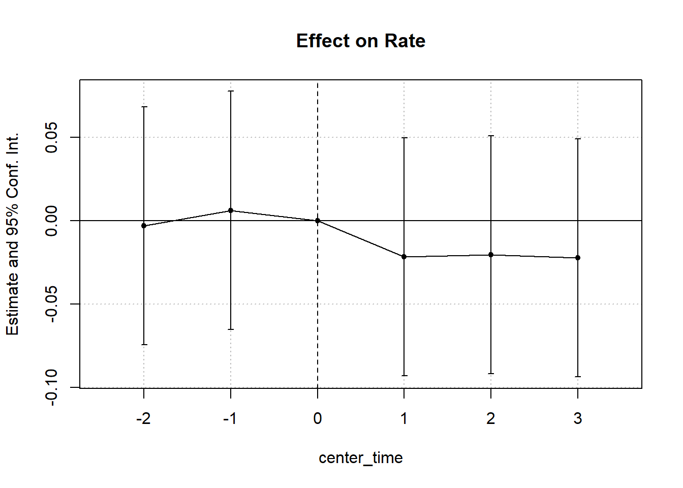

Figure 35.6: Estimated effect on rate over time.

Figure 35.7 shows the same plot with a different plotting function.

coefplot(cali)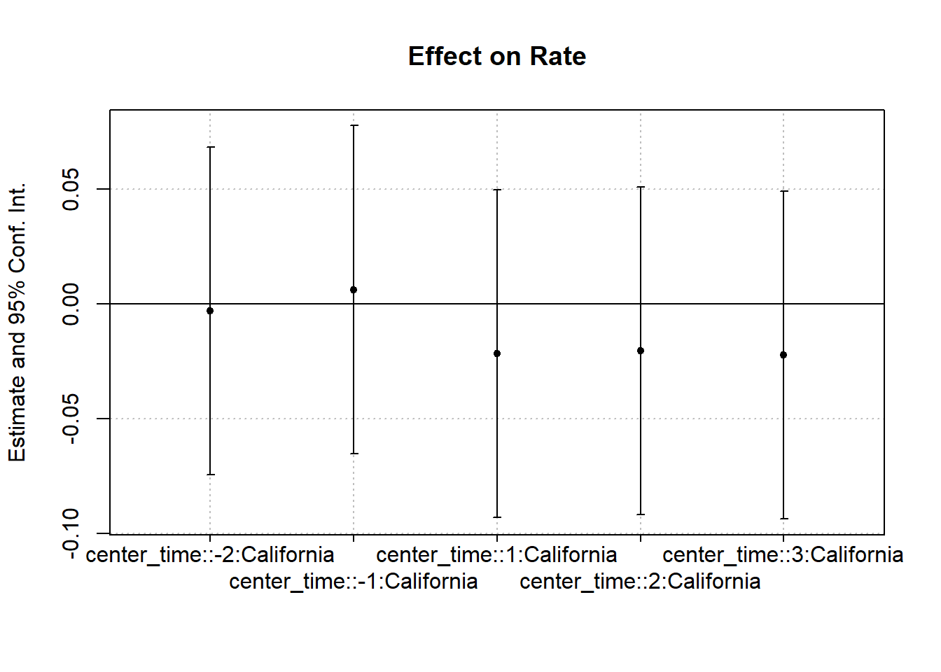

Figure 35.7: Interaction effect on rate.

35.4 Empirical Research Walkthrough

35.4.1 Example: The Unintended Consequences of “Ban the Box” Policies

Doleac and Hansen (2020) examine the unintended effects of “Ban the Box” (BTB) policies, which prevent employers from asking about criminal records during the hiring process. The intended goal of BTB was to increase job access for individuals with criminal records. However, the study found that employers, unable to observe criminal history, resorted to statistical discrimination based on race, leading to unintended negative consequences.

Three Types of “Ban the Box” Policies:

1. Public employers only
2. Private employers with government contracts
3. All employers

Identification Strategy

• If any county within a Metropolitan Statistical Area (MSA) adopts BTB, the entire MSA is considered treated.
• If a state passes a law banning BTB, then all counties in that state are treated.

---

The basic DiD model is:

\[ Y_{it} = \beta_0 + \beta_1 \text{Post}_t + \beta_2 \text{Treat}_i + \beta_3 (\text{Post}_t \times \text{Treat}_i) + \epsilon_{it} \]

where:

• \(Y_{it}\) = employment outcome for individual \(i\) at time \(t\)
• \(\text{Post}_t\) = indicator for post-treatment period
• \(\text{Treat}_i\) = indicator for treated MSAs
• \(\beta_3\) = the DiD coefficient, capturing the effect of BTB on employment
• \(\epsilon_{it}\) = error term

Limitations: If different locations adopt BTB at different times, this model is not valid due to staggered treatment timing.

---

For settings where different MSAs adopt BTB at different times, we use a staggered DiD approach:

\[ \begin{aligned} E_{imrt} &= \alpha + \beta_1 BTB_{imt} W_{imt} + \beta_2 BTB_{mt} + \beta_3 BTB_{mt} H_{imt} \\ &+ \delta_m + D_{imt} \beta_5 + \lambda_{rt} + \delta_m \times f(t) \beta_7 + e_{imrt} \end{aligned} \]

where:

• \(i\) = individual, \(m\) = MSA, \(r\) = region (e.g., Midwest, South), \(t\) = year
• \(W\) = White; \(B\) = Black; \(H\) = Hispanic
• \(BTB_{imt}\) = Ban the Box policy indicator
• \(\delta_m\) = MSA fixed effect
• \(D_{imt}\) = individual-level controls
• \(\lambda_{rt}\) = region-by-time fixed effect
• \(\delta_m \times f(t)\) = linear time trend within MSA

35.4.1.1 Fixed Effects Considerations

• Including \(\lambda_r\) and \(\lambda_t\) separately gives broader fixed effects.

• Using \(\lambda_{rt}\) provides more granular controls for regional time trends.

---

To estimate the effects for Black men specifically, the model simplifies to:

\[ E_{imrt} = \alpha + BTB_{mt} \beta_1 + \delta_m + D_{imt} \beta_5 + \lambda_{rt} + (\delta_m \times f(t)) \beta_7 + e_{imrt} \]

---

To check for pre-trends and dynamic effects, we estimate:

\[ \begin{aligned} E_{imrt} &= \alpha + BTB_{m (t - 3)} \theta_1 + BTB_{m (t - 2)} \theta_2 + BTB_{m (t - 1)} \theta_3 \\ &+ BTB_{mt} \theta_4 + BTB_{m (t + 1)} \theta_5 + BTB_{m (t + 2)} \theta_6 + BTB_{m (t + 3)} \theta_7 \\ &+ \delta_m + D_{imt} \beta_5 + \lambda_{r} + (\delta_m \times f(t)) \beta_7 + e_{imrt} \end{aligned} \]

Key points:

• Leave out \(BTB_{m (t - 1)} \theta_3\) as the reference category (to avoid perfect collinearity).
• If \(\theta_2\) is significantly different from \(\theta_3\), it suggests pre-trend issues, which could indicate anticipatory effects before BTB implementation.

Substantively, Shoag and Veuger (2021) show that Ban-the-box policies increased employment in high-crime neighborhoods by up to 4%, especially in the public sector and low-wage jobs. This is the first nationwide evidence that such laws improve job access for areas with many ex-offenders.

---

35.4.2 Example: Minimum Wage and Employment

Card and Krueger (1993) famously studied the effect of an increase in the minimum wage on employment, challenging the traditional economic view that higher wages reduce employment.

• Philipp Leppert provides an R-based replication.
• Original datasets are available at David Card’s website.

Setting

• Treatment group: New Jersey (NJ), which increased its minimum wage.
• Control group: Pennsylvania (PA), which did not change its minimum wage.
• Outcome variable: Employment levels in fast-food restaurants.

The study used a Difference-in-Differences approach to estimate the impact (Table 35.4).

Table 35.4: DiD estimator illustration using a state-level example.

	State	After (Post)	Before (Pre)	Difference
Treatment	NJ	A	B	A - B
Control	PA	C	D	C - D
		A - C	B - D	(A - B) - (C - D)

where:

• \(A - B\) captures the treatment effect plus general time trends.
• \(C - D\) captures only the general time trends.
• \((A - B) - (C - D)\) isolates the causal effect of the minimum wage increase.

For the DiD estimator to be valid, the following conditions must hold:

1. Parallel Trends Assumption
   • The employment trends in NJ and PA would have been the same in the absence of the policy change.
   • Pre-treatment employment trends should be similar between the two states.
2. No “Switchers”
   • The policy must not induce restaurants to switch locations between NJ and PA (e.g., a restaurant relocating across the border).
3. PA as a Valid Counterfactual
   • PA represents what NJ would have looked like had it not changed the minimum wage.
   • The study focuses on bordering counties to increase comparability.

---

The main regression specification is:

\[ Y_{jt} = \beta_0 + NJ_j \beta_1 + POST_t \beta_2 + (NJ_j \times POST_t)\beta_3+ X_{jt}\beta_4 + \epsilon_{jt} \]

where:

• \(Y_{jt}\) = Employment in restaurant \(j\) at time \(t\)
• \(NJ_j\) = 1 if restaurant is in NJ, 0 if in PA
• \(POST_t\) = 1 if post-policy period, 0 if pre-policy
• \((NJ_j \times POST_t)\) = DiD interaction term, capturing the causal effect of NJ’s minimum wage increase
• \(X_{jt}\) = Additional controls (optional)
• \(\epsilon_{jt}\) = Error term

Notes on Model Specification

• \(\beta_3\) (DiD coefficient) is the key parameter of interest, representing the causal impact of the policy.

• \(\beta_4\) (controls \(X_{jt}\)) is not necessary for unbiasedness but improves efficiency.

• If we difference out the pre-period (\(\Delta Y_{jt} = Y_{j,Post} - Y_{j,Pre}\)), we can simplify the model:

  \[ \Delta Y_{jt} = \alpha + NJ_j \beta_1 + \epsilon_{jt} \]

  Here, we no longer need \(\beta_2\) for the post-treatment period.

---

An alternative specification uses high-wage NJ restaurants as a control group, arguing that they were not affected by the minimum wage increase. However:

• This approach eliminates cross-state differences, but
• It may be harder to interpret causality, as the control group is not entirely untreated.

---

A common misconception in DiD is that treatment and control groups must have the same baseline levels of the dependent variable (e.g., employment levels). However:

• DiD only requires parallel trends, meaning the slopes of employment changes should be the same pre-treatment.
• If pre-treatment trends diverge, this threatens validity.
• If post-treatment trends converge, it may suggest policy effects rather than pre-trend violations.

Is Parallel Trends a Necessary or Sufficient Condition?

• Not sufficient: Even if pre-trends are parallel, other confounders could affect results.
• Not necessary: Parallel trends may emerge only after treatment, depending on behavioral responses.

Thus, we cannot prove DiD is valid. We can only present evidence that supports the assumptions.

---

35.4.3 Example: The Effects of Grade Policies on Major Choice

Butcher et al. (2014) investigate how grading policies influence students’ major choices. The central theory is that grading standards vary by discipline, which affects students’ decisions.

The pattern that the highest-achieving students often concentrate in the hard sciences can be rationalized by two mechanisms.

1. Grading Practices Differ Across Majors
   • In STEM fields, grading is often stricter, meaning professors are less likely to give students the benefit of the doubt.
   • In contrast, softer disciplines (e.g., humanities) may have more lenient grading, raising perceived utility from the major.
2. Labor Market Incentives
   • Degrees with lower market value (e.g., humanities) may compensate by offering a less demanding academic experience.
   • STEM degrees tend to be more rigorous but provide higher job market returns.

---

To examine how grades influence major selection, the study first estimates an OLS model:

\[ E_{ij} = \beta_0 + X_i \beta_1 + G_j \beta_2 + \epsilon_{ij} \]

where:

• \(E_{ij}\) = Indicator for whether student \(i\) chooses major \(j\).
• \(X_i\) = Student-level attributes (e.g., SAT scores, demographics).
• \(G_j\) = Average grade in major \(j\).
• \(\beta_2\) = Key coefficient, capturing how grading standards influence major choice.

Potential Biases in \(\hat{\beta}_2\):

• Negative Bias:
  • Departments with lower enrollment rates may offer higher grades to attract students.
  • This endogenous response leads to a downward bias in the OLS estimate.
• Positive Bias:
  • STEM majors attract the best students, so their grades would naturally be higher if ability were controlled.
  • If ability is not fully accounted for, \(\hat{\beta}_2\) may be upward biased.

---

To address potential endogeneity in OLS, the study uses a difference-in-differences approach:

\[ Y_{idt} = \beta_0 + POST_t \beta_1 + Treat_d \beta_2 + (POST_t \times Treat_d)\beta_3 + X_{idt} + \epsilon_{idt} \]

where:

• \(Y_{idt}\) = Average grade in department \(d\) at time \(t\) for student \(i\).
• \(POST_t\) = 1 if post-policy period, 0 otherwise.
• \(Treat_d\) = 1 if department is treated (i.e., grade policy change), 0 otherwise.
• \((POST_t \times Treat_d)\) = DiD interaction term, capturing the causal effect of grade policy changes on major choice.
• \(X_{idt}\) = Additional student controls.

---

Table 35.5: Group-level design matrix for difference-in-differences.

Group	Intercept (\(\beta_0\))	Treatment (\(\beta_2\))	Post (\(\beta_1\))	Interaction (\(\beta_3\))
Treated, Pre	1	1	0	0
Treated, Post	1	1	1	1
Control, Pre	1	0	0	0
Control, Post	1	0	1	0

Table 35.5 shows how we can think about the design matrix for DID.

• The average pre-period outcome for the control group is given by \(\beta_0\).
• The key coefficient of interest is \(\beta_3\), which captures the difference in the post-treatment effect between treated and control groups.

---

A more flexible specification includes fixed effects:

\[ Y_{idt} = \alpha_0 + (POST_t \times Treat_d) \alpha_1 + \theta_d + \delta_t + X_{idt} + u_{idt} \]

where:

• \(\theta_d\) = Department fixed effects (absorbing \(Treat_d\)).
• \(\delta_t\) = Time fixed effects (absorbing \(POST_t\)).
• \(\alpha_1\) = Effect of policy change (equivalent to \(\beta_3\) in the simpler model).

Why Use Fixed Effects?

• More flexible specification:
  • Instead of assuming a uniform treatment effect across groups, this model allows for department-specific differences (\(\theta_d\)) and time-specific shocks (\(\delta_t\)).
• Higher degrees of freedom:
  • Fixed effects absorb variation that would otherwise be attributed to \(POST_t\) and \(Treat_d\), making the estimation more efficient.

Interpretation of Results

• If \(\alpha_1 > 0\), then the policy increased grades in treated departments.
• If \(\alpha_1 < 0\), then the policy decreased grades in treated departments.

---

35.5 One Difference

The regression formula is as follows Liaukonytė et al. (2023):

\[ y_{ut} = \beta \text{Post}_t + \gamma_u + \gamma_w(t) + \gamma_l + \gamma_g(u)p(t) + \epsilon_{ut} \]

where

• \(y_{ut}\): Outcome of interest for unit u in time t.
• \(\text{Post}_t\): Dummy variable representing a specific post-event period.
• \(\beta\): Coefficient measuring the average change in the outcome after the event relative to the pre-period.
• \(\gamma_u\): Fixed effects for each unit.
• \(\gamma_w(t)\): Time-specific fixed effects to account for periodic variations.
• \(\gamma_l\): Dummy variable for a specific significant period (e.g., a major event change).
• \(\gamma_g(u)p(t)\): Group x period fixed effects for flexible trends that may vary across different categories (e.g., geographical regions) and periods.
• \(\epsilon_{ut}\): Error term.

This model can be used to analyze the impact of an event on the outcome of interest while controlling for various fixed effects and time-specific variations, but using units themselves pre-treatment as controls.

---

35.6 Two-Way Fixed Effects

A generalization of the Difference-in-Differences model is the two-way fixed effects (TWFE) model, which accounts for multiple groups and multiple time periods by including both unit and time fixed effects. In practice, TWFE is frequently used to estimate causal effects in panel data settings. However, it is not a design-based, non-parametric causal estimator (Imai and Kim 2021), and it can suffer from severe biases if the treatment effect is heterogeneous across units or time.

When applying TWFE to datasets with multiple treatment groups and staggered treatment timing, the estimated causal coefficient is a weighted average of all possible two-group, two-period DiD comparisons. Crucially, some of these weights can be negative (Goodman-Bacon 2021), which leads to potential biases. The weighting scheme depends on:

• Group sizes
• Variation in treatment timing
• Placement in the middle of the panel (units in the middle tend to get the highest weight)

---

35.6.1 Canonical TWFE Model

The canonical TWFE model is typically written as:

\[ Y_{it} = \alpha_i + \lambda_t + \tau W_{it} + \beta X_{it} + \epsilon_{it}, \]

where:

• \(Y_{it}\) = Outcome for unit \(i\) at time \(t\)

• \(\alpha_i\) = Unit fixed effect

• \(\lambda_t\) = Time fixed effect

• \(\tau\) = Causal effect of treatment

• \(W_{it}\) = Treatment indicator (\(1\) if treated, \(0\) otherwise)

• \(X_{it}\) = Covariates

• \(\epsilon_{it}\) = Error term

An illustrative TWFE event-study model (Stevenson and Wolfers 2006):

\[ \begin{aligned} Y_{it} &= \sum_{k} \beta_{k} \cdot Treatment_{it}^{k} + \eta_{i} + \lambda_{t} + Controls_{it} + \epsilon_{it}, \end{aligned} \]

where:

• \(Treatment_{it}^k\): Indicator for whether unit \(i\) is in its \(k\)-th year relative to treatment at time \(t\).

• \(\eta_i\): Unit fixed effects, controlling for time-invariant unobserved heterogeneity.

• \(\lambda_t\): Time fixed effects, capturing overall macro shocks.

• Standard Errors: Typically clustered at the group or cohort level.

Usually, researchers drop the period immediately before treatment (\(k=-1\)) to avoid collinearity. However, dropping this or another period inappropriately can shift or bias the estimates.

When there are only two time periods \((T=2)\), TWFE simplifies to the traditional DiD model. Under homogeneous treatment effects and if the parallel trends assumption holds, \(\hat{\tau}_{OLS}\) is unbiased. Specifically, the model assumes (Imai and Kim 2021):

1. Homogeneous treatment effects across units and time periods, meaning:
   • No dynamic treatment effects (i.e., treatment effects do not evolve over time).
   • The treatment effect is constant across units (Goodman-Bacon 2021; De Chaisemartin and d’Haultfoeuille 2020; Sun and Abraham 2021; Borusyak et al. 2024).
2. Parallel trends assumption
3. Linear additive effects are valid (Imai and Kim 2021).

However, in practice, treatment effects are often heterogeneous. If effects vary by cohort or over time, then standard TWFE estimates can be biased, particularly when there is staggered adoption or dynamic treatment effects (Goodman-Bacon 2021; De Chaisemartin and d’Haultfoeuille 2020; Sun and Abraham 2021; Borusyak et al. 2024). Hence, to use the TWFE, we actually have to argue why the effects are homogeneous to justify TWFE use:

• Assess treatment heterogeneity: If heterogeneity exists, TWFE may produce biased estimates. Researchers should:
  • Plot treatment timing across units.
  • Decompose the treatment effect using the Goodman-Bacon decomposition to identify negative weights.
  • Check the proportion of never-treated observations: When 80% or more of the sample is never treated, TWFE bias is negligible.
  • Beware of bias worsening with long-run effects.
• Dropping relative time periods:
  • If all units eventually receive treatment, two relative time periods must be dropped to avoid multicollinearity.
  • Some software packages drop periods randomly; if a post-treatment period is dropped, bias may result.
  • The standard approach is to drop periods -1 and -2.
• Sources of treatment heterogeneity:
  • Delayed treatment effects: The impact of treatment may take time to manifest.
  • Evolving effects: Treatment effects can increase or change over time (e.g., phase-in effects).

---

TWFE compares different types of treatment/control groups:

• Valid comparisons:
  • Newly treated units vs. control units
  • Newly treated units vs. not-yet treated units
• Problematic comparisons:
  • Newly treated units vs. already treated units (since already treated units do not represent the correct counterfactual).
  • Strict exogeneity violations:
    • Presence of time-varying confounders
    • Feedback from past outcomes to treatment (Imai and Kim 2019)
  • Functional form restrictions:
    • Assumes treatment effect homogeneity.
    • No carryover effects or anticipation effects (Imai and Kim 2019).

---

35.6.2 Limitations of TWFE

TWFE inherits its appeal from a deceptively simple promise: absorb unit and time effects, and the residual variation that survives identifies the causal coefficient. That promise holds when treatment effects are constant. Once effects vary across units or evolve over time, the residual variation no longer maps cleanly onto a single causal quantity. The price of using a one-coefficient model on a many-coefficient world shows up as bias, not as obvious model failure, which is why these limitations were under-appreciated for years.

The strong assumptions that TWFE rides on can be enumerated as follows:

• No dynamic treatment effects: The model requires that the treatment effect not evolve over time.
• No unit-level differences: The treatment effect must be constant across all units.
• Linear additive effects: TWFE assumes that the underlying data-generating process is captured by additive fixed effects plus a constant treatment effect (Imai and Kim 2021).

If any of these assumptions are violated, TWFE can produce biased estimates. The mechanics of the bias are worth pausing on, because they motivate every modern remedy discussed below. When treatment is staggered, the regression coefficient is an implicit average of many smaller two-by-two comparisons, and the weights attached to those comparisons are determined by panel structure rather than by what the researcher cares about. Symptoms include:

• Negative weights and biased estimates: With multiple groups and staggered timing, the TWFE estimate becomes a complicated average of “two-group, two-period” DiD comparisons, some of which can receive negative weights (Goodman-Bacon 2021).
• Bias from dropped relative-time periods: If all units eventually get treated, software often drops a reference period (or periods) to avoid multicollinearity. If the dropped period is post-treatment, the bias can worsen. Researchers often drop relative time \(-1\) or \(-2\).
• Delayed or evolving treatment effects: If the effect of treatment takes time to manifest or changes over time, TWFE’s single coefficient \(\tau\) can be misleading.

When two time periods only exist, TWFE collapses back to the traditional DiD model, making these problems far less severe. But as soon as one moves beyond a single treatment period or has variation in treatment timing, these issues become critical. The same logic surfaces in Multiple Periods and Variation in Treatment Timing, where staggered adoption is the rule rather than the exception, and these failure modes have spawned a whole generation of estimators (see Modern Estimators for Staggered Adoption and Modern Concerns in DiD).

Several authors (Sun and Abraham 2021; Callaway and Sant’Anna 2021; Goodman-Bacon 2021) have catalogued concrete pathologies of TWFE DiD regressions under staggered adoption:

• Cohort mixing: The regression unintentionally compares newly treated units to already treated units, conflating post-treatment behavior of early adopters with the pre-treatment trends of later adopters.
• Negative weights: Some group comparisons receive negative weights, which can reverse the sign of the overall estimate.
• Spurious pre-treatment leads: Leads may appear non-zero if earlier-treated groups remain in the sample as implicit “controls” while later adopters are still untreated.
• Compounding long-run bias: Heterogeneity in lagged (long-run) effects accumulates as the panel lengthens, so longer windows do not necessarily produce cleaner estimates.

The empirical stakes are substantial. In fields such as finance and accounting, newer estimators often reveal null or much smaller effects than standard TWFE once bias is properly accounted for (Baker et al. 2022). Substantial portions of these literatures have had to revisit headline results, which underscores the importance of the diagnostics in the next subsection.

---

35.6.3 Diagnosing and Addressing Bias in TWFE

Before reaching for a sophisticated alternative estimator, it pays to ask how badly TWFE is actually misbehaving in the design at hand. The diagnostics below answer that question with progressively heavier machinery, beginning with a picture of the data and ending with a formal decomposition of the regression coefficient itself. Researchers should treat these as a sequence: a quick visual check tells you whether to worry, the share of never-treated units tells you how much room there is for negative weights, and the Goodman-Bacon Decomposition tells you which two-by-two comparisons are doing the damage.

1. Goodman-Bacon Decomposition

• Purpose: Decomposes the TWFE DiD estimate into the sum of all two-group, two-period comparisons.
• Insight: Reveals which comparisons have negative weights and how much each comparison contributes to the overall estimate (Goodman-Bacon 2021).
• Implementation: Identify subgroups by treatment timing, then examine each group-time pair to see how it contributes to the aggregate TWFE coefficient.
• When it is decisive: If the decomposition shows that “already-treated as control” comparisons receive substantial weight, TWFE is structurally compromised and a remedy from the next subsection is warranted.

2. Plotting Treatment Timing

• Visual inspection: Always plot the distribution of treatment timing across units.
• High risk of bias: If treatment is staggered and many units differ in their adoption times, standard TWFE will often be biased.
• Cheap and informative: This step takes minutes, costs nothing, and frequently changes which estimator a careful researcher reaches for next.

3. Assessing Treatment Heterogeneity Directly

• Check for variation in effects: If there is a theoretical or empirical reason to believe that treatment effects differ by subgroup or over time, TWFE might not be appropriate.
• Size of never-treated sample: When 80% or more of the sample is never treated, the potential for bias in TWFE is smaller because the regression leans heavily on clean treated-versus-never-treated comparisons. Large shares of treated units with varied adoption times raise red flags.
• Long-run effects: Bias can worsen if the treatment effect accumulates or changes over time, since the coefficient on the treatment indicator averages early and late dynamics with weights chosen by the panel rather than by the researcher.

If the diagnostics suggest that TWFE is mildly biased, an event-study specification with carefully chosen reference periods may suffice. If they suggest a structural problem, the remedies in the next subsection become necessary rather than optional.

---

35.6.3.1 Goodman-Bacon Decomposition

The Goodman-Bacon decomposition (Goodman-Bacon 2021) is a powerful diagnostic tool for understanding the TWFE estimator in settings with staggered treatment adoption. This approach clarifies how the TWFE DiD estimate is a weighted average of many 2×2 difference-in-differences comparisons between groups treated at different times (or never treated).

Key Takeaways

• A pairwise DiD estimate (\(\tau\)) receives more weight when:
  • The treatment happens closer to the midpoint of the observation window.
  • The comparison involves more observations (e.g., more units or more years).
• Comparisons between early-treated and later-treated groups can produce negative weights, potentially biasing the aggregate TWFE estimate.

We illustrate the decomposition using the castle dataset from the bacondecomp package:

library(bacondecomp)
library(tidyverse)

# Load and inspect the castle dataset
castle <- bacondecomp::castle %>% 
  dplyr::select(l_homicide, post, state, year)
head(castle)
#>   l_homicide post   state year
#> 1   2.027356    0 Alabama 2000
#> 2   2.164867    0 Alabama 2001
#> 3   1.936334    0 Alabama 2002
#> 4   1.919567    0 Alabama 2003
#> 5   1.749841    0 Alabama 2004
#> 6   2.130440    0 Alabama 2005

Running the Goodman-Bacon Decomposition

# Apply Goodman-Bacon decomposition
df_bacon <- bacon(
  formula = l_homicide ~ post,
  data = castle,
  id_var = "state",
  time_var = "year"
)
#>                       type  weight  avg_est
#> 1 Earlier vs Later Treated 0.05976 -0.00554
#> 2 Later vs Earlier Treated 0.03190  0.07032
#> 3     Treated vs Untreated 0.90834  0.08796

# Display weighted average of the decomposition
weighted_avg <- sum(df_bacon$estimate * df_bacon$weight)
weighted_avg
#> [1] 0.08181162

Comparing with the TWFE Estimate

library(broom)

# Fit a TWFE model
fit_tw <- lm(l_homicide ~ post + factor(state) + factor(year), data = castle)
tidy(fit_tw)
#> # A tibble: 61 × 5
#>    term                     estimate std.error statistic   p.value
#>    <chr>                       <dbl>     <dbl>     <dbl>     <dbl>
#>  1 (Intercept)                1.95      0.0624    31.2   2.84e-118
#>  2 post                       0.0818    0.0317     2.58  1.02e-  2
#>  3 factor(state)Alaska       -0.373     0.0797    -4.68  3.77e-  6
#>  4 factor(state)Arizona       0.0158    0.0797     0.198 8.43e-  1
#>  5 factor(state)Arkansas     -0.118     0.0810    -1.46  1.44e-  1
#>  6 factor(state)California   -0.108     0.0810    -1.34  1.82e-  1
#>  7 factor(state)Colorado     -0.696     0.0810    -8.59  1.14e- 16
#>  8 factor(state)Connecticut  -0.785     0.0810    -9.68  2.08e- 20
#>  9 factor(state)Delaware     -0.547     0.0810    -6.75  4.18e- 11
#> 10 factor(state)Florida      -0.251     0.0798    -3.14  1.76e-  3
#> # ℹ 51 more rows

Interpretation: The TWFE estimate (approx. 0.08) equals the weighted average of the Bacon decomposition estimates, confirming the decomposition’s validity.

---

Visualizing the Decomposition (Figure 35.8)

library(ggplot2)

ggplot(df_bacon) +
  aes(
    x = weight,
    y = estimate,
    color = type
  ) +
  geom_point() +
  labs(
    x = "Weight",
    y = "Estimate",
    color = "Comparison Type"
  ) +
  causalverse::ama_theme()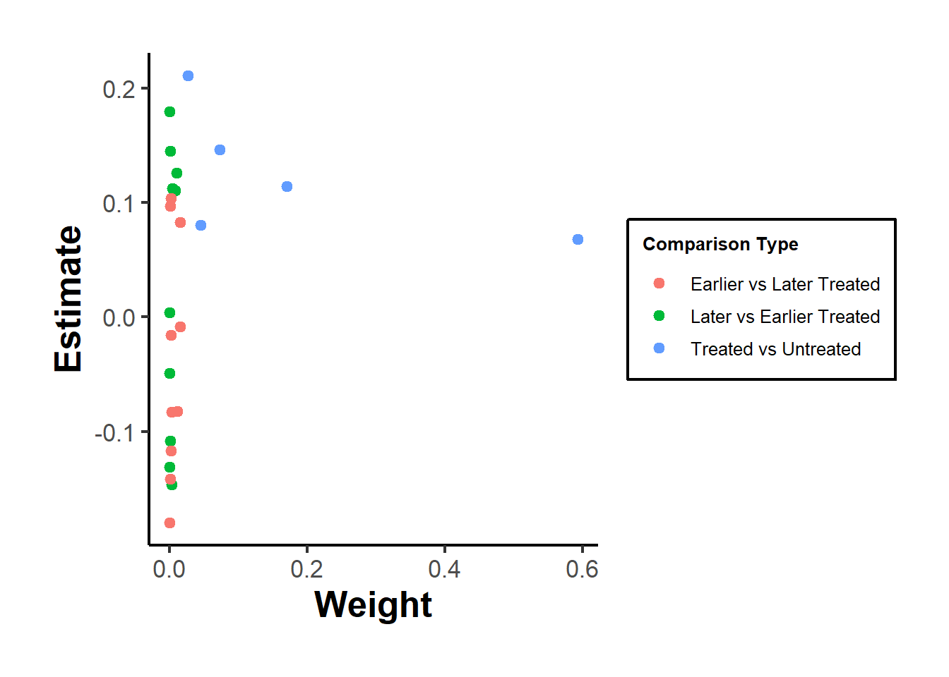

Figure 35.8: Decomposition of treatment effects by comparison type and weight.

Insight: This plot shows the contribution of each 2×2 DiD comparison, highlighting how estimates with large weights dominate the overall TWFE coefficient.

---

Interpretation and Practical Implications

• Purpose: Decomposes the TWFE DiD estimate into the sum of all two-group, two-period comparisons.
• Insight: Reveals how much each comparison contributes to the overall estimate and whether any have negative or misleading effects.
• Implementation:
  • Identify subgroups by treatment timing.
  • Compute DiD for each 2×2 comparison (early vs. late, late vs. never, etc.).
  • Evaluate how these contribute to the final TWFE estimate.

When time-varying covariates are included that allow for identification within treatment timing groups, certain problematic comparisons (like “early vs. late”) may no longer influence the TWFE estimator directly. These scenarios may collapse into simpler within-group estimates, improving identification (Table 35.6).

Table 35.6: Goodman-Bacon comparison types.

Comparison Type	Description	Common Issue
Treated vs. Never	Clean comparisons if never-treated units exist	Often reliable
Early vs. Late	Later group is control in earlier period	May introduce bias
Late vs. Early	Early group is control in later period	May reverse causality
Treated vs. Treated	Within-treatment variation by timing	Sensitive to dynamics

---

35.6.4 Remedies for TWFE’s Shortcomings

The estimators surveyed here all share a single ambition: recover an interpretable average treatment effect when treatment is staggered, treatment effects are heterogeneous, and dynamics matter. They differ in what data they need, what they assume, and what they deliver. Rather than treat the list as a menu of independent tools, it helps to keep three questions in mind while reading. First, does the design have a meaningful pool of never-treated (or not-yet-treated) units? Second, do treatment effects evolve with exposure length, and is that dynamic itself the object of interest? Third, can units toggle treatment on and off, or is treatment an absorbing state? The answers narrow the field quickly and motivate the cross-references at the end of the subsection (see also Modern Estimators for Staggered Adoption and Modern Concerns in DiD).

The core idea uniting the estimators below is to disaggregate the single TWFE coefficient into well-defined building blocks (typically group-time or cohort-time effects), estimate each block from comparisons that are guaranteed to be clean, and only then aggregate using transparent weights. Stated this way, modern DiD looks less like a zoo of competing methods and more like one strategy with several flavors.

1. Group-Time Average Treatment Effects

Callaway and Sant’Anna (2021) propose a two-step approach:

1. Group-time treatment effects: In each time period, estimate the effect for the cohort that first received treatment in that period (compared to a never-treated group).
2. Aggregate: Use a bootstrap procedure to account for autocorrelation and clustering, then aggregate across groups.

• Advantages: Allows for heterogeneous treatment effects across groups and over time; compares treated groups only with never-treated units (or well-chosen controls).
• When it dominates: This is often the default first move when the panel contains a credible never-treated (or not-yet-treated) comparison group and the researcher wants to summarize effects flexibly across cohorts and exposure lengths.
• What its assumptions cost: It needs parallel trends to hold conditional on the chosen comparison group and is most informative when each cohort has enough mass to estimate cohort-specific effects with reasonable precision.
• Implementation: did package in R.

2. Event-Study Design with Cohort-Specific Estimates

Sun and Abraham (2021) build on Callaway and Sant’Anna (2021) to handle event-study settings:

• Lags and leads: Capture dynamic treatment effects by including time lags and leads relative to the event (treatment).
• Cohort-specific estimates: Estimate separate paths of outcomes for each cohort, controlling for other cohorts carefully.
• Interaction-weighted estimator: Adjusts for differences in when treatment began.
• When it dominates: Choose this when the dynamic path of the effect (the shape of the event study) is the substantive question and standard event-study coefficients in TWFE are contaminated by other cohorts’ treatment effects bleeding into the leads and lags.
• Implementation: fixest package in R.

3. Panel Match DiD Estimator with In-and-Out Treatment Conditions

Imai and Kim (2021) develop methods allowing units to switch in and out of treatment:

• Matching to create a weighted version of TWFE, addressing some of the bias from heterogeneous effects.
• When it dominates: This is the natural choice when treatment is reversible (units enter and exit) so absorbing-state estimators do not apply, and when the researcher is comfortable arguing for conditional ignorability given an observed history. It connects DiD to the broader logic of matching on pre-treatment trajectories.
• Implementation: wfe and PanelMatch R packages.

4. Two-Stage Difference-in-Differences (DiD2S)

Gardner (2022) propose two-stage DiD:

• Idea: Partial out fixed effects first, then perform a second-stage regression that focuses on within-group/time variation.
• Strength: Handles heterogeneous treatment effects well, especially when never-treated units are present.
• When it dominates: It offers a computationally light path to consistent staggered-DiD estimates with familiar regression output, useful when researchers want to incorporate covariates flexibly without committing to the full machinery of cohort-time aggregation.
• Implementation: did2s R package.

5. Switching DiD Estimator

• If a study has never-treated units, De Chaisemartin and d’Haultfoeuille (2020) suggest an switching DiD estimator to recover the average treatment effect.
• When it dominates: Particularly useful when researchers care about a single, period-specific average effect among switchers rather than a full event-time profile.
• Caveat: This approach still fails to detect heterogeneity if treatment effects vary with exposure length (Sun and Shapiro 2022), so pair it with a dynamic specification when long-run effects are plausible.

6. Matrix Completion Estimator

This estimator imputes missing potential outcomes for treated cells by fitting a low-rank structure to the panel, much like the synthetic control and synthetic difference-in-differences approaches it is conceptually related to. It comes into its own when the panel is wide (many units, many periods), parallel trends across simple cohort groupings looks implausible, and a flexible counterfactual model is preferable to a strict comparison-group design (see also counterfactual estimators).

7. Reshaped Inverse Probability Weighting-TWFE Estimator

• Design-based approaches: Arkhangelsky et al. (2024) offer further refinements that incorporate inverse probability weighting.
• Goal: Improve balance and reduce bias from non-random treatment timing.
• When it dominates: Useful when researchers want to keep the convenience of a TWFE-style regression but fear that the weights TWFE implicitly applies are misaligned with the target estimand. The reweighting recasts the estimand as a design-based object, trading some efficiency for a more credible interpretation.

8. Stacked DiD (simpler but biased)

• Build stacked datasets for each treatment cohort, running separate regressions for each “event window.”
• This approach is simpler but can still carry biases if the underlying assumptions are violated (Gormley and Matsa 2011; Cengiz et al. 2019; Deshpande and Li 2019).
• When it dominates: It is often the right pragmatic first pass in industry settings or when communicating to audiences uncomfortable with cohort-time aggregation, since each stacked panel reduces to a familiar two-by-two comparison. Treat it as a cousin of the formal staggered-DiD estimators above rather than a substitute, and always cross-check against one of them.

9. Doubly Robust Difference-in-Differences Estimators (DR-DID) (Sant’Anna and Zhao 2020)

• DR-DID estimators combine outcome regression and propensity score weighting to identify treatment effects, remaining consistent if either model is correctly specified.
• They achieve local efficiency under joint correctness and can be applied to both panel and repeated cross-section data.
• When it dominates: Ideal when covariate adjustment is essential (the conditional ignorability and overlap assumptions are doing real work) and the researcher wants insurance against misspecification of either the outcome or the treatment model.

10. Nonlinear Difference-in-Differences

• When the outcome is binary, count, or otherwise bounded, additive parallel trends can be implausible because shifts at one part of the distribution mechanically constrain shifts elsewhere. Nonlinear DiD addresses this by working on a transformed scale or by directly modeling the distribution. See also Changes-in-Changes and the comparison in CIC vs Quantile DiD.

A practical decision logic ties these threads together. If the panel has a reliable never-treated group and the question is “what is the average effect across cohorts and exposure lengths,” start with Callaway and Sant’Anna (2021) and use Sun and Abraham (2021) when the dynamic path is the focus. If treatment toggles on and off, switch to the panel-matching family of Imai and Kim (2021). If covariates carry most of the identifying weight, prefer a doubly robust estimator. If the panel is wide and parallel trends is hard to defend on raw data, lean on counterfactual estimators such as matrix completion or synthetic difference-in-differences. Stacked DiD and TWFE remain useful as exposition tools and pragmatic baselines, but should not stand alone as the headline estimator under staggered adoption.

---

35.6.5 Best Practices and Recommendations

The recommendations below collapse the preceding diagnostic and remedy discussions into a workflow. The order matters: confirm whether TWFE is even defensible for the design, diagnose bias before reaching for alternatives, tune the event-study specification to avoid self-inflicted artifacts, and only then graduate to a modern estimator if the diagnostics warrant it. The same logic underlies the more detailed treatment in Modern Estimators for Staggered Adoption.

1. When is TWFE Appropriate?
   • Single treatment period: TWFE DiD works well if there is only one treatment period for all treated units (no variation in timing). In that special case it reduces to the simple DiD and the staggered-adoption pathologies vanish.
   • Homogeneous effects: If strong theoretical or empirical reasons suggest constant treatment effects across cohorts and over time, TWFE remains a reasonable choice. The argument for homogeneity should be made explicitly and defended, not assumed by default.
2. Diagnosing and Addressing Bias with Staggered Adoption
   • Plot treatment timing: Examine the distribution of treatment timing across units (see Visualization). If treatment adoption is highly staggered, TWFE is likely to produce biased estimates.
   • Decomposition methods: Use the Goodman-Bacon Decomposition (Goodman-Bacon 2021) to see how TWFE pools comparisons (and whether negative weights emerge). If decomposition is infeasible (e.g., unbalanced panels), the share of never-treated units can indicate potential bias severity.
     • Decomposes the TWFE DiD estimate into two-group, two-period comparisons.
     • Identifies which comparisons receive negative weights, which can lead to biased estimates.
     • Helps determine the influence of specific groups on the overall estimate.
   • Discuss heterogeneity: Explicitly state the likelihood of treatment effect heterogeneity and incorporate it into the research design rather than treating it as a footnote.
3. Event-Study Specifications within TWFE
   • Avoid arbitrary binning: Do not collapse multiple time periods into a single bin unless you can justify homogeneous effects within that bin.
   • Full relative-time indicators: Include flexible event-time indicators, carefully choosing a reference period (commonly \(-1\), the year before treatment). Specifically, include fully flexible relative time indicators and justify the reference period (usually \(l = -1\) or the period just prior to treatment).
   • Beware of multicollinearity: Including leads and lags can cause multicollinearity and artificially produce significant “pre-trends.”
   • Drop the right periods: If all units eventually get treated, dropping post-treatment periods accidentally can bias results.
4. Consider Alternative Estimators: If the diagnostics flag staggered adoption with non-trivial heterogeneity, move to one of the modern estimators discussed above. Robustness checks across several modern estimators (see also Robustness Checks and Modern Concerns in DiD) are now the norm in careful applied work, since agreement across methods that lean on different assumptions is the strongest evidence the result is not an artifact of any one specification.

---

35.7 Multiple Periods and Variation in Treatment Timing

TWFE has been extended beyond the simple DiD setup to multiple periods and staggered adoption (where treatment occurs at different times for different units). Such designs are common in applied economics, public policy, and longitudinal research. However, standard TWFE regressions can be biased in these contexts when treatment effects are heterogeneous across groups or over time.

35.7.1 Staggered Difference-in-Differences

In staggered treatment adoption (also called event-study DiD or dynamic DiD):

• Different units adopt the treatment at different time periods.
• Standard TWFE often produces biased estimates because it “pools” all treated units (regardless of when they started treatment) together, implicitly comparing newly treated units to already treated ones.
• Treatments that occurred earlier may contaminate the counterfactual for later adopters if the model does not properly handle dynamic or heterogeneous effects (Wing et al. 2024; Baker et al. 2022).
• For applied guidance, see (Wing et al. 2024) and recommendations in (Baker et al. 2022).

Researchers should be aware that standard TWFE can mix treatment effects of early adopters (long-exposed) with later adopters (newly exposed), potentially assigning negative weights to particular group comparisons (Goodman-Bacon 2021).

When using staggered adoption, the following assumptions are critical:

1. Rollout Exogeneity
   Treatment assignment and timing should be uncorrelated with potential outcomes.

   • Evidence: Regress adoption on pre-treatment variables. And if you find evidence of correlation, include linear trends interacted with pre-treatment variables (Hoynes and Schanzenbach 2009)
   • Evidence (Deshpande and Li 2019, 223):
     • Treatment is random: Regress treatment status at the unit level to all pre-treatment observables. If you have some that are predictive of treatment status, you might have to argue why it’s not a worry. At best, you want this.
     • Treatment timing is random: Conditional on treatment, regress timing of the treatment on pre-treatment observables. At least, you want this.

2. No Confounding Events
   Ensure no other policies or shocks coincide with the staggered treatment rollout.

3. Exclusion Restrictions

   • No Anticipation: Treatment timing should not affect outcomes prior to treatment.
   • Invariance to History: Treatment duration shouldn’t matter; only the treated status matters (often violated).

4. Standard DID Assumptions

   • Parallel Trends (Conditional or Unconditional)
   • Random Sampling
   • Overlap (Common Support)
   • Effect Additivity

---

35.8 Bayesian Difference-in-Differences

Notation in this section follows the conventions of Table 31.12 in the foundations chapter.

The standard Difference-in-Differences estimator is a frequentist device. It produces a point estimate of the treatment effect, an estimated standard error, and a confidence interval whose coverage is justified by appeals to repeated sampling. This machinery works well when the panel is large, the treatment timing is common, and the analyst is content to report a single number with an interval around it. The Bayesian formulation of DiD keeps the identifying logic intact, the same parallel-trends reasoning underwrites the design, but replaces the inferential apparatus with a posterior distribution over the quantities of interest. Instead of a point estimate and a standard error, the analyst obtains a full distribution for the average treatment effect on the treated, for any cohort-specific or period-specific effect, and for any function of these that a decision maker might care about.

This reframing pays off in three situations that recur in applied work. When the panel is small, so that asymptotic normal approximations are unreliable, the posterior propagates finite-sample uncertainty honestly rather than relying on a sandwich estimator whose justification is asymptotic. When effects are heterogeneous across many cohorts or units, partial pooling shares information across them in a way that disciplines noisy cohort-level estimates without forcing them to a common value. And when the analyst must feed the treatment effect into a downstream decision, an inventory choice, a pricing rule, a regulatory cost-benefit calculation, the posterior delivers exactly the object that decision theory requires, namely a probability distribution over the unknown effect that can be integrated against a loss function.

35.8.1 From the two-way fixed-effects regression to a probability model

Recall the canonical regression form of DiD with a single treatment onset. For unit \(i\) observed in period \(t\),

\[ Y_{it} \;=\; \alpha_i \;+\; \gamma_t \;+\; \tau\, W_{it} \;+\; \varepsilon_{it}, \]

where \(\alpha_i\) is a unit fixed effect, \(\gamma_t\) is a period fixed effect, \(W_{it}\) indicates active treatment, and \(\tau\) is the treatment effect. Frequentist DiD estimates this by least squares and treats \(\tau\) as a fixed unknown constant.

The Bayesian version writes the same mean structure but completes it into a generative probability model by specifying a sampling distribution for the outcome and prior distributions for every parameter. A typical specification is

\[ \begin{aligned} Y_{it} \mid \alpha_i, \gamma_t, \tau &\;\sim\; \mathcal{N}\!\bigl(\alpha_i + \gamma_t + \tau\, W_{it},\; \sigma^2\bigr), \\ \alpha_i &\;\sim\; \mathcal{N}\!\bigl(\mu_\alpha,\; \sigma_\alpha^2\bigr), \\ \gamma_t &\;\sim\; \mathcal{N}\!\bigl(\mu_\gamma,\; \sigma_\gamma^2\bigr), \\ \tau &\;\sim\; \mathcal{N}\!\bigl(0,\; \sigma_\tau^2\bigr), \end{aligned} \]

with weakly informative hyperpriors on the variance components such as half-normal or half-Student-t distributions on \(\sigma\), \(\sigma_\alpha\), \(\sigma_\gamma\) (Gelman 2006). Two features distinguish this from the frequentist regression. First, the unit and period effects are now drawn from common distributions rather than being free parameters; this is the random-effects or partial-pooling structure that the Bayesian framework handles naturally. Second, the treatment effect \(\tau\) carries its own prior, which the analyst chooses to reflect substantive knowledge about plausible effect magnitudes.

Inference targets the posterior distribution

\[ p\bigl(\tau, \boldsymbol{\alpha}, \boldsymbol{\gamma}, \sigma, \ldots \mid \mathbf{Y}\bigr) \;\propto\; p\bigl(\mathbf{Y} \mid \tau, \boldsymbol{\alpha}, \boldsymbol{\gamma}, \sigma\bigr)\, p(\tau)\, p(\boldsymbol{\alpha})\, p(\boldsymbol{\gamma})\, p(\sigma)\, \cdots, \]

which is summarized by drawing samples through Hamiltonian Monte Carlo (Gelman et al. 2013). From those draws, the posterior for \(\tau\) alone is obtained by marginalizing over the nuisance parameters, which Monte Carlo accomplishes simply by ignoring the other coordinates of each draw.

35.8.2 Priors on treatment effects

The prior on \(\tau\) is the most visible modeling choice, and it deserves care rather than reflexive vagueness. A flat or extremely diffuse prior reproduces the frequentist point estimate in large samples but offers no regularization when data are thin and can place substantial prior mass on absurd effect sizes. A weakly informative prior, by contrast, encodes the order of magnitude that the outcome scale permits, a treatment that doubles sales is plausible, one that multiplies them by a thousand is not, without committing to a particular value.

For continuous outcomes measured on a standardized scale, a normal prior centered at zero with a standard deviation chosen to span the range of credible effects is a common default. Centering at zero is not an assertion that the effect is zero; it expresses the prior judgment that small effects are more likely than large ones and lets the data move the posterior away from zero when the evidence warrants. When prior studies or a meta-analysis supply a credible range for the effect, that information can be encoded directly in the prior, which is one of the clearest advantages of the Bayesian approach over an analysis that discards such evidence. The sensitivity of conclusions to the prior should always be reported, ideally by re-running the model under a small set of defensible priors and showing that the substantive conclusion is stable, or by being explicit about where it is not.

35.8.3 Partial pooling for heterogeneous and staggered effects

The setting where the Bayesian framework earns its keep is the modern staggered-adoption design, where units adopt treatment at different times and the effect may differ by adoption cohort and by time since adoption. The frequentist literature has documented that the naive two-way fixed-effects regression delivers a treatment-effect estimate that is a weighted average of cohort-by-period effects with weights that can be negative, producing estimates that need not lie in the convex hull of the underlying effects (Goodman-Bacon 2021; Sun and Abraham 2021; Callaway and Sant’Anna 2021). The recommended frequentist remedy is to estimate each cohort-by-period effect separately and then aggregate with sensible nonnegative weights.

The Bayesian analogue estimates the disaggregated effects but adds a hierarchical layer that pools them. Let \(\tau_{g,e}\) denote the effect for cohort \(g\) (the group that adopts in period \(g\)) at event time \(e\) (periods since adoption). A hierarchical model writes

\[ \begin{aligned} \tau_{g,e} &\;\sim\; \mathcal{N}\!\bigl(\theta_e,\; \omega^2\bigr), \\ \theta_e &\;\sim\; \mathcal{N}\!\bigl(\mu_\theta,\; \kappa^2\bigr), \end{aligned} \]

so that each cohort’s effect at event time \(e\) is shrunk toward a common event-time profile \(\theta_e\), and the profile itself is regularized. The degree of shrinkage is not chosen by the analyst but learned from the data through the posterior for \(\omega\): when the cohort effects are similar, \(\omega\) is estimated small and the model pools aggressively; when they genuinely differ, \(\omega\) is large and the model lets each cohort speak for itself. This adaptive pooling is the central practical benefit. Cohorts with few treated units, which would yield hopelessly noisy standalone estimates, borrow strength from better-identified cohorts, while cohorts with abundant data are barely shrunk. The same logic underlies the broader literature on hierarchical Bayesian models in panel and small-area settings (Gelman and Hill 2006).

Once the posterior for the full set of \(\tau_{g,e}\) is in hand, any aggregate of interest is a deterministic function of the draws and inherits a posterior automatically. The overall average treatment effect on the treated is a cohort-size-weighted average of the relevant \(\tau_{g,e}\); its posterior is obtained by computing that weighted average within each Monte Carlo draw. Event-study coefficients, the average effect over a horizon, and the difference between early and late adopters are all handled the same way, with no separate delta-method or bootstrap step required.

35.8.4 Posterior inference and credible intervals

The output of the analysis is a set of posterior draws for every parameter and for every derived quantity. Reporting proceeds by summarizing these draws. The posterior mean or median of \(\tau\) serves as a point summary, and a credible interval, for instance the central interval spanning the 2.5th to 97.5th posterior percentiles, communicates uncertainty. A 95 percent credible interval has the interpretation that practitioners often wrongly attach to a confidence interval, namely that, conditional on the model and prior, there is a 95 percent posterior probability that the effect lies in the interval. Because the interval is read off the posterior directly, it requires no appeal to asymptotic normality and remains valid in small samples where a normal-approximation confidence interval would mislead.

The posterior also answers questions that a confidence interval cannot pose. The posterior probability that the effect exceeds a managerially relevant threshold, the probability that early adopters benefited more than late adopters, or the probability that the effect is positive in at least one cohort are each computed as the fraction of draws satisfying the condition. These probability statements map cleanly onto the decisions that motivate most applied DiD studies.

Model adequacy is assessed through posterior predictive checks, simulating replicated datasets from the fitted model and comparing them to the observed data, and through convergence diagnostics for the sampler such as the potential scale reduction factor and effective sample size (Gelman et al. 2013). For DiD specifically, the pre-treatment fit deserves scrutiny: the model’s implied pre-treatment trajectories for treated and control units should track the data, since a model that misfits the pre-period offers no reason to trust its counterfactual in the post-period. This is the Bayesian counterpart of the pre-trends check that disciplines any DiD analysis.

35.8.5 Advantages and costs

The advantages cluster around three themes. First, uncertainty is represented coherently and completely: every quantity, no matter how complicated a function of the parameters, comes with a posterior, and finite-sample uncertainty is propagated without asymptotic approximation. Second, the hierarchical structure is a natural fit for staggered and heterogeneous designs, delivering adaptive partial pooling that stabilizes noisy cohort-level estimates while letting genuine heterogeneity surface. Third, prior information, whether from earlier studies, a meta-analysis, or domain expertise, can be incorporated transparently rather than discarded, which is especially valuable when the panel is short.

These benefits are not free. The analyst must specify priors and defend them, the computation through Markov chain Monte Carlo is heavier than a single regression and requires convergence checks, and the inferences are conditional on the model in a way that places the burden on careful model checking. The Bayesian and frequentist analyses typically agree when data are abundant and priors are weak; they diverge, and the Bayesian treatment tends to be more honest, precisely in the small-sample and many-cohort regimes where the asymptotic frequentist story is least credible.

35.8.6 Implementation

The brms package provides a formula interface to Stan that expresses these models compactly (Bürkner 2017), while rstanarm offers precompiled models for common cases (Goodrich et al. 2020). The chunk below sketches a hierarchical staggered-DiD specification; it is not evaluated here because it requires a compiled Stan toolchain and a fitted panel.

library(brms)

# panel: outcome y, unit id, period t, cohort g, event time e (NA pre-treatment),
# treatment indicator w (1 when actively treated)

# Two-way fixed effects with a single treatment effect and weakly informative priors
fit_simple <- brm(
    y ~ w + (1 | id) + (1 | t),
    data   = panel,
    prior  = c(
        prior(normal(0, 1),       class = "b",  coef = "w"),
        prior(student_t(3, 0, 2), class = "sd"),
        prior(student_t(3, 0, 2), class = "sigma")
    ),
    chains = 4, cores = 4, iter = 2000, seed = 1
)

# Hierarchical staggered design: cohort-by-event-time effects pooled toward an
# event-time profile via a varying-slope term over event time within cohort
fit_staggered <- brm(
    y ~ 1 + (1 | id) + (1 | t) + (1 + factor(e) | g),
    data   = subset(panel, !is.na(e)),
    prior  = c(
        prior(student_t(3, 0, 2), class = "sd"),
        prior(student_t(3, 0, 2), class = "sigma")
    ),
    chains = 4, cores = 4, iter = 2000, seed = 1
)

# Posterior summaries and a credible interval for the treatment effect
summary(fit_simple)
posterior_interval(fit_simple, pars = "b_w", prob = 0.95)

# Posterior probability that the effect exceeds a decision threshold
draws <- as_draws_df(fit_simple)
mean(draws$b_w > 0.10)

The first model recovers a single treatment effect with partial pooling on the unit and period intercepts. The second lets each cohort carry its own event-time profile while shrinking those profiles toward a common shape, which is the disaggregate-then-pool strategy that the staggered-DiD literature recommends, implemented in one coherent probability model.

35.9 Nonparametric Difference-in-Differences and Latent Factor Models

Notation in this section follows the conventions of Table 31.12 in the foundations chapter.

This section develops methods for identifying and estimating average treatment effects in a panel-data setting without relying on strong functional-form assumptions. The standard two-way fixed-effects (TWFE) model and the linear factor model impose linearity or additivity on the unobserved unit-specific and time-specific components, which makes them easy to implement but restrictive. The framework here allows fully nonparametric relationships between potential outcomes, latent unit factors, latent time factors, and idiosyncratic shocks. The goal is to estimate the Average Treatment Effect on the Treated under considerably weaker functional-form assumptions than a TWFE regression requires, within a panel that permits unobserved heterogeneity in both the cross-sectional and the time dimensions.

The intellectual lineage runs through the nonlinear difference-in-differences model of Athey and Imbens (2006) and the nonparametric fixed-effects panel regression of Lee and Robinson (2015), both of which loosen the additive-linear structure that the textbook DiD imposes. We build on that foundation by treating the unit and time effects as latent factors that enter the outcome through an unknown function.

35.9.1 Setup and potential outcomes

A typical two-way fixed-effects model posits, for the untreated outcome of unit \(i\) in period \(t\),

\[ Y_{it}(0) \;=\; \alpha_i + \beta_t + \varepsilon_{it}, \]

with \(\alpha_i\) a unit effect, \(\beta_t\) a time effect, and \(\varepsilon_{it}\) an idiosyncratic shock. This additive structure is ubiquitous in applied work, but it can fail when the relationship between the latent components and the outcome is genuinely nonlinear or non-additive. A nonparametric panel model relaxes the additivity while retaining the factor structure, letting the latent components enter through a flexible unknown function subject only to mild smoothness and separability conditions.

Consider a panel of \(N\) units (individuals, firms, or regions) observed over \(T\) periods, \(t \in \{1, \ldots, T\}\). Let \(W_{it} \in \{0,1\}\) denote treatment status. The two potential outcomes are \(Y_{it}(0)\), the outcome if untreated, and \(Y_{it}(1)\), the outcome if treated, with the realized outcome

\[ Y_{it} = \begin{cases} Y_{it}(0), & W_{it} = 0, \\ Y_{it}(1), & W_{it} = 1. \end{cases} \]

The target estimand is the average treatment effect on the treated,

\[ \tau \;=\; \mathrm{ATT} \;=\; \frac{\sum_{i,t} W_{it}\,\bigl[Y_{it}(1) - Y_{it}(0)\bigr]}{\sum_{i,t} W_{it}}, \]

the average effect over the treated cell pairs \((i,t)\). Because \(Y_{it}(0)\) is unobserved for treated cells, identifying \(\tau\) is a missing-data problem.

The classical DiD design supposes two periods and two groups and invokes parallel trends for the untreated potential outcomes, the multi-period analogue of the linear TWFE model. As soon as one allows nonlinear dependence of outcomes on the latent factors, or non-parallel trends driven by time effects that vary across units in a non-additive way, standard DiD and TWFE become biased. The nonparametric factor framework is the natural generalization that does not lean on linearity or parallel trends.

35.9.2 Nonparametric factor model

Let the untreated potential outcome arise from an unknown function \(g(\cdot)\) of three arguments,

\[ Y_{it}(0) \;=\; g\bigl(\alpha_i,\; \beta_t,\; \varepsilon_{it}\bigr), \]

where \(\alpha_i \in \mathcal{A} \subseteq \mathbb{R}^{d_\alpha}\) is a random vector specific to unit \(i\), \(\beta_t \in \mathcal{B} \subseteq \mathbb{R}^{d_\beta}\) is a random vector specific to period \(t\), and \(\varepsilon_{it}\) is an idiosyncratic error that may be correlated over time within a unit but is independent across units. We impose no linearity, additivity, or parametric form on \(g\). Instead we require three conditions.

First, smoothness: \(g(\alpha, \beta, \varepsilon)\) is continuously differentiable, or at least Hölder continuous, with uniformly bounded first derivatives. Second, latent independence: the collections \(\{\alpha_i\}\), \(\{\beta_t\}\), and \(\{\varepsilon_{it}\}\) are mutually independent, with \(\alpha_i\) independent and identically distributed across units; the time factor \(\beta_t\) may be autocorrelated provided its marginal distribution is stationary, and likewise for the shocks. Third, both \(N\) and \(T\) grow large in the asymptotic sequence, so that additional observations fill in the matrix rather than expand it, in the spirit of the infill asymptotics familiar from time-series and spatial econometrics (Zhang and Zimmerman 2005).

One motivation for the factor-separable structure is row-and-column exchangeability from random-matrix theory, which guarantees a representation of the form \(g(\alpha_i, \beta_t, \varepsilon_{it})\). We simply posit that such a representation exists and exploit its factor structure for identification. Two familiar models are nested as special cases. Two-way fixed effects corresponds to \(g(\alpha_i, \beta_t, \varepsilon_{it}) = \alpha_i + \beta_t + \varepsilon_{it}\), and the linear factor model corresponds to \(g(\alpha_i, \beta_t, \varepsilon_{it}) = \alpha_i^\top \beta_t + \varepsilon_{it}\), the interactive-fixed-effects structure that underlies the generalized synthetic control method (Xu 2017) and the dynamic interactive-effects estimators of Moon and Weidner (2017). The nonparametric model does not restrict \(g\) to be linear, additive, or even low rank, requiring only that it depend on unit-specific and time-specific factors and on an idiosyncratic shock.

When a unit is treated at \((i,t)\), its potential outcome is

\[ Y_{it}(1) \;=\; g\bigl(\alpha_i, \beta_t, \varepsilon_{it}\bigr) + \delta(\alpha_i, \beta_t), \]

where \(\delta(\alpha, \beta)\) is the structural treatment increment, which may itself depend on the latent factors. The individual effect is then \(Y_{it}(1) - Y_{it}(0) = \delta(\alpha_i, \beta_t)\), and

\[ \tau \;=\; \frac{\sum_{i,t} W_{it}\, \delta(\alpha_i, \beta_t)}{\sum_{i,t} W_{it}}. \]

Because \(\alpha_i\) and \(\beta_t\) are unobserved, we cannot condition on them directly, which is the core identification challenge.

35.9.3 Identifying assumptions

To impute the counterfactual \(Y_{it}(0)\) for treated cells we need a design restriction on how treatment is assigned. In a cross-sectional observational study, unconfoundedness requires \(W_i \perp Y_i(0)\) conditional on observed covariates \(X_i\). Here the relevant confounders are the latent factors, so we impose latent-factor ignorability.

The first component is latent-factor unconfoundedness,

\[ \{W_{it}\} \;\perp\; Y_{it}(0) \;\bigm|\; (\alpha_i, \beta_t), \]

which states that conditional on the latent unit factor and latent time factor, treatment assignment is as good as random for that cell. The second component is overlap: there exists a constant \(c > 0\) such that

\[ 0 < c \;\le\; \Pr\bigl(W_{it} = 1 \mid \alpha_i, \beta_t\bigr) \;\le\; 1 - c < 1 \]

for all latent values, so that every cell has a nontrivial chance of being treated and of being untreated given its factors. The third is the stable unit treatment value assumption, ruling out interference and hidden versions of treatment.

If \(\alpha_i\) and \(\beta_t\) were observed, these conditions would reduce to ordinary unconfoundedness. The point is that they are not observed: we see only \((Y_{it}, W_{it})\). The factor structure ensures that two units sharing the same or similar \(\alpha\)-value have untreated outcomes that behave similarly across all times, and symmetrically for the time factors. Because the latent factors are never seen, these assumptions cannot be tested directly and must be defended on design or domain grounds.

Under these conditions, identification reduces to learning the conditional mean of the untreated outcome,

\[ \mu(\alpha, \beta) \;=\; E\bigl[g(\alpha, \beta, \varepsilon) \mid \alpha, \beta\bigr]. \]

If \(\mu(\alpha_i, \beta_t)\) can be recovered for each treated cell, then \(Y_{it}(0)\) can be imputed and the ATT follows by averaging \(Y_{it}(1) - \mu(\alpha_i, \beta_t)\) over the treated cells. We need neither identify \(\alpha_i\) and \(\beta_t\) themselves nor recover the full function \(g\); we need only the expected untreated outcome at the relevant factor values.

35.9.4 Identification through covariance-based matching

The obstacle is that \(\alpha_i\) and \(\beta_t\) are latent, so we cannot condition on them. The key insight is that units with similar functions \(\mu(\alpha_i, \cdot)\) over \(\beta\) can serve as matches for one another, and that this similarity is detectable from the data through co-movement over time. If two units \(i\) and \(j\) have similar entire functions \(\mu(\alpha_i, \cdot)\) and \(\mu(\alpha_j, \cdot)\), then for any third unit \(k\) the covariance patterns of \((Y_{it}, Y_{kt})\) and \((Y_{jt}, Y_{kt})\) across \(t\) will be close.

To make this precise at the population level, define for any pair of unit types \(\alpha, \alpha'\) the discrepancy

\[ \Gamma(\alpha, \alpha') \;=\; E_\beta\Bigl[\bigl(\mu(\alpha, \beta) - \mu(\alpha', \beta)\bigr)^2\Bigr]. \]

When \(\Gamma(\alpha, \alpha') = 0\), the functions \(\mu(\alpha, \cdot)\) and \(\mu(\alpha', \cdot)\) coincide almost everywhere in \(\beta\), so \(\alpha\) and \(\alpha'\) are equivalent unit types for the untreated potential outcome. We never observe \(\alpha_i\), but the discrepancy can be expanded into cross-covariance terms,

\[ \Gamma(\alpha, \alpha') \;=\; E_\beta\Bigl[\bigl(\mu(\alpha, \beta) - \mu(\alpha', \beta)\bigr)\,\mu(\alpha, \beta)\Bigr] - E_\beta\Bigl[\bigl(\mu(\alpha, \beta) - \mu(\alpha', \beta)\bigr)\,\mu(\alpha', \beta)\Bigr], \]

so that verifying \(\Gamma(\alpha, \alpha') = 0\) amounts to checking that the difference \(\mu(\alpha, \beta) - \mu(\alpha', \beta)\) is uncorrelated with \(\mu(\alpha'', \beta)\) for every type \(\alpha''\). With large \(N\), the observed units supply a dense set of probe types \(\alpha''\), and with large \(T\) the sample covariances converge to their population counterparts.

This motivates a feasible empirical matching set. For each unit \(i\) and a tolerance \(\nu > 0\), define

\[ \mathcal{J}_\nu(i) \;=\; \Bigl\{ j \ne i : \max_{k \ne i,j} \bigl|\,\widehat{\mathrm{Cov}}_t\bigl(Y_{it} - Y_{jt},\, Y_{kt}\bigr)\,\bigr| \;\le\; \nu \Bigr\}, \]

where \(\widehat{\mathrm{Cov}}_t(X_t, Z_t) = \tfrac{1}{T}\sum_{t}(X_t - \bar{X})(Z_t - \bar{Z})\). The set collects units \(j\) whose differenced time profile relative to \(i\) is nearly uncorrelated with every other unit’s profile, which strongly suggests \(\mu(\alpha_i, \beta) \approx \mu(\alpha_j, \beta)\) across \(\beta\). As \(\nu \to 0\) the set shrinks toward truly similar units, and as \(N, T \to \infty\), under Lipschitz conditions on \(g\) and uniform convergence of the sample covariances, each unit acquires at least one match while \(\mu(\alpha_i, \cdot) \approx \mu(\alpha_j, \cdot)\) in sup norm. Choosing \(\nu\) to shrink slowly with the sample size balances these forces. The ordinary matching that suffices in the TWFE setting fails in this more general model, which is precisely why the covariance-based construction is needed.

35.9.5 Estimating the ATT

Given \(\mathcal{J}_\nu(i)\), restrict to the matches that are in the control condition at period \(t\), \(\mathcal{J}_\nu(i,t) = \{ j \in \mathcal{J}_\nu(i) : W_{jt} = 0 \}\), and impute the untreated outcome by averaging over them,

\[ \hat{Y}_{it}(0) \;=\; \frac{1}{|\mathcal{J}_\nu(i,t)|} \sum_{j \in \mathcal{J}_\nu(i,t)} Y_{jt}. \]

By the overlap assumption, with probability approaching one some matches remain untreated at \(t\), so the set is nonempty and \(\hat{Y}_{it}(0)\) approximates \(\mu(\alpha_i, \beta_t)\). For each treated cell the individual effect is estimated by \(\hat{\delta}_{it} = Y_{it} - \hat{Y}_{it}(0)\), and aggregating over treated cells gives

\[ \hat{\tau} \;=\; \frac{\sum_{(i,t):\,W_{it}=1}\bigl[Y_{it} - \hat{Y}_{it}(0)\bigr]}{\sum_{i,t} W_{it}}. \]

Under the regularity conditions above, \(\hat{\tau}\) converges in probability to the ATT. The estimator never invokes a parametric form for \(\mu(\alpha_i, \beta_t)\) nor a parallel-trends restriction; it relies instead on conditional unconfoundedness given the latent factors, recovered through matching.

35.9.6 Relation to other models

When \(g(\alpha_i, \beta_t, \varepsilon_{it}) = \alpha_i + \beta_t + \varepsilon_{it}\), the conditional mean is additive, \(\mu(\alpha_i, \beta_t) = \alpha_i + \beta_t\). Covariance-based matching then selects units with the same \(\alpha\)-value, because in the additive case any difference in unit types shows up as a level difference regardless of how the time factor moves. Differencing out \(\alpha_i\) or \(\beta_t\) is feasible, and the procedure collapses to ordinary DiD or a TWFE regression. Once \(\mu\) is non-additive, the differencing argument breaks and the matching approach is the correct generalization.

The linear factor model \(g(\alpha_i, \beta_t, \varepsilon_{it}) = \alpha_i^\top \beta_t + \varepsilon_{it}\) is the other leading special case. Estimators in that tradition, such as the interactive-fixed-effects approach of Moon and Weidner (2017), the generalized synthetic control method of Xu (2017), and the factor-model causal estimator of Li and Sonnier (2023), recover \(\alpha_i\) and \(\beta_t\) under assumptions on the shock process. The nonparametric model does not estimate the factors directly; it treats them as latent random variables and works around them through matching.

35.9.7 Practical considerations and extensions

In large panels, scanning \(\max_{k \ne i,j} |\widehat{\mathrm{Cov}}(\cdots)|\) over all pairs costs on the order of \(N^3 T\) operations. A common remedy is to cluster the units first, for instance by an approximate factor structure recovered through a singular value decomposition or by the grouped-heterogeneity device that assumes \(\alpha_i\) takes finitely many values, and then to match finely within clusters. Regularization, such as imposing a bandwidth or stopping once enough matches are found, avoids the search for an exact covariance match.

Staggered adoption requires care: for each treated cell there must be enough matches that remain untreated at that period, so overlap must hold period by period. If nearly every unit is treated by some date, the approach loses its footing in those periods.

For inference, \(\hat{\tau}\) behaves like a matching estimator, and the factor dependence complicates the usual variance formulas. A block bootstrap that resamples entire unit time series, or entire periods, preserves the cross-sectional and temporal dependence; one recomputes the match sets and the estimator within each draw and reads off the sampling distribution of \(\hat{\tau}\). Under the large-\(N\), large-\(T\) regularity conditions the bootstrap recovers the correct limiting distribution.

The same factor-matching machinery extends beyond causal inference to decomposition exercises. In an Oaxaca-Blinder decomposition of a between-group gap (Oaxaca 1973; Blinder 1973), let \(W_{it} = 1\) index membership in one group and \(W_{it} = 0\) the other. The mean outcome gap decomposes into an explained component, attributable to differences in the distributions of the latent factors across groups, and an unexplained component, attributable to differences in the conditional-mean function \(\mu\) itself,

\[ \underbrace{E\bigl[\mu_1(\alpha^1, \beta^1)\bigr] - E\bigl[\mu_0(\alpha^0, \beta^0)\bigr]}_{\text{gap}} = \underbrace{E\bigl[\mu_1(\alpha^1, \beta^1)\bigr] - E\bigl[\mu_0(\alpha^1, \beta^1)\bigr]}_{\text{unexplained}} + \underbrace{E\bigl[\mu_0(\alpha^1, \beta^1)\bigr] - E\bigl[\mu_0(\alpha^0, \beta^0)\bigr]}_{\text{explained}}. \]

Although the factors remain unobserved, the same matching argument imputes the counterfactual “what if one group had the other group’s distribution of latent factors,” provided each group’s factor structure is stable within group. The logic that identifies a treatment effect thus also identifies a group-membership decomposition.

35.10 Temporal Causal Inference with Staggered Cohorts

Notation in this section follows the conventions of Table 31.12 in the foundations chapter.

The difference-in-differences designs developed so far all rely on the existence of a control group that escapes the treatment, at least for a while. A policy hits one set of states and not another, a price change reaches one market and not its neighbor, a product feature ships to a treated arm and not a holdout. The hard case arises when an event reaches everyone at once. A publicly announced data breach, a recall, a regulatory ruling, or a viral news story is known to the entire population almost simultaneously, so there is no contemporaneous group of unaware units to serve as a control. Traditional experimental and quasi-experimental tools, A/B tests, randomized trials, test markets, and conventional DiD, all presuppose a clean comparison group, and that group simply does not exist after a widely known shock. Even if one could find units that somehow remained unaware, they would be unrepresentative of the population precisely because they missed the event.

Temporal causal inference, proposed by Turjeman and Feinberg (2023), resolves this by constructing the control group from the same population at an earlier point in its own history rather than from a different population at the same calendar time. The idea exploits the fact that, when an event strikes, different units are at different stages of their lifecycle or tenure. A user who joined a service three weeks before a breach experiences the shock early in their engagement; a user who joined three years earlier experiences it deep into a mature relationship. If behavior follows a trajectory that depends mainly on tenure rather than on calendar time, then the early-tenure experience of a long-standing cohort, observed before the event reached them, predicts what the treated short-tenure cohort would have done absent the event.

35.10.1 From staggered tenure to treated and control cohorts

The design reorganizes the panel along tenure, the time since a unit first adopted or joined, rather than along calendar time. Let \(H_T\) denote the cohort of participants who joined exactly \(T\) time units before the event occurred. For this treated cohort, the event lands \(T\) units into their tenure, and the analyst observes their behavior for a window that extends some periods past the event, capturing the post-event response.

The control group for \(H_T\) is assembled from cohorts \(H_1, \ldots, H_{T-1}\) that joined earlier and therefore reached tenure \(T\) before the event arrived. For each such earlier cohort, the analyst tracks activity from first adoption up to the point where the event reaches them or the observation window closes, whichever comes first. The crucial property is that these earlier cohorts passed through tenure \(T\), the tenure at which the treated cohort meets the event, while the event had not yet occurred for them. Their behavior at that tenure therefore furnishes the counterfactual: it is what the treated cohort would have done at tenure \(T\) had the event not happened.

A subtlety is that every cohort is eventually exposed to the event, since the shock is population-wide. The control cohorts are not unexposed; they are exposed later in their own tenure. The design uses only the segment of each control cohort’s trajectory that precedes its own exposure, so within the comparison window the control observations are genuinely event-free. Most cohorts play both roles across the analysis, serving as controls for later-joining cohorts and as treated units relative to earlier ones; only the very earliest and very latest cohorts in the window are confined to a single role.

The plot below illustrates the construction with several simulated cohorts. The upper panel shows behavior against calendar time, where the cohorts are shifted horizontally because they joined at different dates. The lower panel realigns them against tenure, the time since each cohort’s own adoption, which is the axis on which the cohorts become comparable. Aligned on tenure, the cohorts trace similar trajectories, and the treated cohort meets the event at the tenure where the earlier cohorts had not yet been exposed.

library(ggplot2)
library(patchwork)

# Base tenure grid shared by every cohort
tenure <- seq(0, 99, length.out = 100)

# Each cohort joins at a different calendar time but follows a tenure-driven path
generate_cohort <- function(name, start_time, mean, sd) {
    data.frame(
        tenure = tenure,
        cohort = name,
        time   = seq(start_time, start_time + 99, by = 1),
        value  = dnorm(tenure, mean = mean, sd = sd)
    )
}

cohorts <- list(
    generate_cohort("Cohort 1", 1,  47, 15),
    generate_cohort("Cohort 2", 10, 48, 17),
    generate_cohort("Cohort 3", 20, 52, 20),
    generate_cohort("Cohort 4", 30, 53, 18),
    generate_cohort("Treated",  40, 50, 16)
)
final_dataset <- do.call(rbind, cohorts)

# Calendar-time view: cohorts are offset because they joined on different dates
plot_time <-
    ggplot(final_dataset, aes(x = time, y = value, color = cohort)) +
    geom_line(linewidth = 0.7) +
    geom_vline(xintercept = 40, linetype = "dashed") +
    geom_vline(xintercept = 90, linetype = "dashed") +
    labs(title = "Behavior vs. calendar time", x = "Time", y = "Value") +
    theme_minimal()

# Tenure view: aligned on time since adoption, the cohorts become comparable
plot_tenure <-
    ggplot(final_dataset, aes(x = tenure, y = value, color = cohort)) +
    geom_line(linewidth = 0.7) +
    geom_vline(xintercept = 0,  linetype = "dashed") +
    geom_vline(xintercept = 50, linetype = "dashed") +
    labs(title = "Behavior vs. tenure", x = "Tenure", y = "Value") +
    theme_minimal()

plot_time / plot_tenure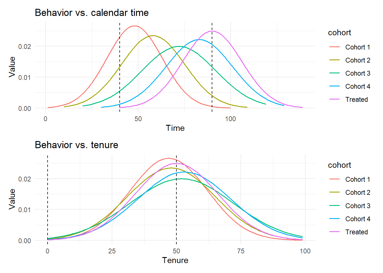

The upper panel displays behavior over calendar time for one treated cohort and several earlier cohorts. The lower panel realigns the same series on tenure, showing that the cohorts share a common shape once tenure is held fixed; the control cohorts have not yet met the event at the tenure where the treated cohort encounters it.

Before any model, it pays to show model-free evidence, the simple average of the outcome for treated and control groups around the event. The chunk below reproduces that descriptive comparison from the data accompanying Turjeman and Feinberg (2023); it is not evaluated here because it depends on study-specific labeling that lives outside this book’s build.

percent_active_per_group <- rio::import(file.path(
    getwd(), "data", "mksc.2019.0208", "percent_active_per_group.csv"
))

ggplot(percent_active_per_group,
       aes(x = time_from, y = avg_avg, linetype = as.factor(group_type))) +
    geom_line(linewidth = 0.75) +
    geom_vline(xintercept = 0) +
    scale_y_continuous(labels = scales::percent_format(accuracy = 1)) +
    scale_linetype_manual(values = c("dotted", "solid")) +
    labs(x = "Weeks from treatment",
         y = "Average percent of active users",
         linetype = "Group") +
    theme_minimal()

35.10.2 Potential outcomes and the role of multiple control cohorts

The framework is the usual potential-outcomes one. For each unit there is an outcome absent the event, \(Y_i(0)\), and an outcome with the event, \(Y_i(1)\), only one of which is observed; the unobserved counterfactual is imputed as \(\hat{Y}_i(0)\) or \(\hat{Y}_i(1)\), and the probability of exposure is estimated as \(\hat{w}_i \in (0,1)\). What distinguishes temporal causal inference is the source of the counterfactual: rather than a single contemporaneous control group, it draws on many control cohorts that joined at distinct times.

This multiplicity is a strength. Each control cohort lived through the comparison tenure window during a different calendar interval, so any cohort-specific calendar disturbance, a seasonal swing, a competitor’s promotion, a macroeconomic wobble, contaminates only the cohorts active during that interval. Averaging the counterfactual across many cohorts that span different calendar intervals averages out these idiosyncratic disturbances, leaving the tenure-driven component that the design is built to recover. A single control group offers no such averaging.

35.10.3 Identifying assumptions

Temporal causal inference rests on the same assumptions as other selection-on-observables designs, reinterpreted for the tenure-aligned cohort structure.

The stable unit treatment value assumption has two parts. The first is no interference between units. Because treated and control cohorts are defined by tenure and observed during non-overlapping segments of calendar time within the comparison window, a unit’s assignment does not act on another unit’s outcome through the usual contemporaneous channels: for a pair \(\{i, j\}\) in different cohorts, \(Y_i(1) \perp Y_j(0)\) within the window. After a population-wide shock, treated units may influence one another, so \(Y_i(1)\) and \(Y_j(1)\) need not be independent across all treated pairs; the design confines attention to comparisons where this is least problematic. The second part is no hidden versions of treatment, so that the observed outcome is \(Y_i = W_i Y_i(1) + (1 - W_i) Y_i(0)\) and only the event of interest moves the outcome. This is hard to guarantee outside a controlled trial, but using many control cohorts that joined at different dates dilutes the influence of any single extraneous event on the imputed \(Y_i(0)\), since unrelated disturbances are averaged across cohorts.

Conditional independence, or ignorability, requires that assignment to the treated or control role be independent of the potential outcomes given covariates, \(P(W_i \mid X_i, Y_i(0), Y_i(1)) = P(W_i \mid X_i)\). Here assignment is governed by join time, the tenure at which a unit met the event, so the concern is whether the date a unit joined is related to its outcome trajectory in a way the covariates do not capture. The design validates the implied parallel-trends condition empirically. A bidirectional Granger test checks whether the control series helps predict the treated series and vice versa in the pre-event window, with the goal of finding the two statistically indistinguishable before the event. A Kolmogorov-Smirnov test compares the pre-event timelines of the two groups to confirm they are drawn from comparable distributions. Passing both supports the claim that, prior to the event, treated and control cohorts were on the same path.

Overlap requires a treatment propensity strictly between zero and one for every unit given covariates, \(0 < \Pr(W_i = 1 \mid X_i = x) < 1\). In this design every unit is eventually treated, and at any given tenure each unit had a positive chance of being on either side of the event, so overlap is plausible; it can be examined directly through the estimated propensity \(\hat{w}(x)\).

Finally, exogeneity of covariates requires that the covariates not be affected by the event. This is supported when the shock is genuinely unforeseen. If some units anticipated it, the anticipation is likely shared across treated and control cohorts, so the design controls for it and identification of the treatment effect is preserved.

35.10.4 Relation to staggered difference-in-differences

Temporal causal inference is closely related to, but distinct from, the staggered DiD designs of the preceding sections. Staggered DiD estimates treatment effects when an intervention reaches different units at different calendar times and at least some units remain untreated as controls within each period; the analyst aligns on calendar time and exploits the staggering of adoption. Temporal causal inference inverts the geometry. The event reaches everyone at nearly the same calendar moment, so there is no contemporaneous holdout, and the staggering that the design exploits is in tenure rather than in adoption of the treatment. By realigning cohorts on tenure and using earlier cohorts’ pre-event tenure segments as the counterfactual, it manufactures a control group out of the population’s own history. When a clean contemporaneous control group exists, staggered DiD is the natural tool; when the shock is population-wide and no such group exists, temporal causal inference supplies the comparison that DiD cannot.

As with any matching or nonparametric design, the method is data-hungry. Stable trajectory matching across cohorts, credible Granger and Kolmogorov-Smirnov diagnostics, and well-estimated propensities all require many units per cohort and a reasonably long tenure window. With thin cohorts the imputed counterfactual is noisy and the pre-event diagnostics lose power, so the approach is best suited to settings with large panels of individually tracked units.

35.11 Instrumented Difference-in-Differences

Notation in this section follows the conventions of Table 31.12 in the foundations chapter.

The parallel-trends assumption that licenses ordinary difference-in-differences is an assumption about untreated potential outcomes: absent the treatment, the treated and control groups would have moved on parallel paths. A common reason this fails is that the groups differ not only in treatment but in the trajectory of the exposure itself, and that the divergent exposure trend is driven by unobserved factors whose influence varies over time. When the trend in the outcome diverges because the trend in exposure diverges, ordinary DiD attributes the gap to the treatment and is biased. Instrumented difference-in-differences, developed by Ye et al. (2022), addresses exactly this situation by introducing an instrument that perturbs the exposure trend without acting on the outcome trend directly.

The motivating design is a longitudinal study, possibly with repeated cross-sections, in which an encouragement is delivered after a baseline period to push units toward taking the treatment regularly. The encouragement plays the role of an instrument for the trend in exposure. If the encouragement has no direct effect on the trend in the outcome, then any nonparallel trend in the outcome that tracks the nonparallel trend in exposure can be ascribed to the treatment. The method thereby converts a violation of parallel trends, caused by differential exposure, into an identification opportunity.

35.11.1 What the instrument buys

Two features distinguish instrumented DiD from both ordinary DiD and standard instrumental variables. First, it is robust to time-varying unmeasured confounding of the exposure-outcome relationship. The instrument, the encouragement, is by construction independent of the time-varying unmeasured confounders, so confounding that is time-invariant but has time-varying effects, or that is itself time-varying, does not bias the estimate. Ordinary DiD cannot tolerate this, because such confounding is what breaks parallel trends in the first place.

Second, the exclusion restriction is weaker than in a conventional instrumental-variables analysis. A standard IV must have no direct effect on the outcome at all. The encouragement in instrumented DiD is permitted to have a direct effect on the outcome level, provided it does not affect the outcome trend and does not modify the treatment effect. This is a meaningful relaxation. Consider a firm testing a new pricing strategy on sales, while also offering loyalty-program discounts to some customers. As a standard instrument the discount fails, since it raises sales directly. But it may still serve as an instrument for DiD if the pricing strategy’s effect differs across loyalty and non-loyalty customers over time while the discount offered to each group stays constant over time. Variables that shift levels but not trends are therefore candidate instruments for DiD even when they are invalid as standard instruments. A further practical advantage over fuzzy DiD is that units may switch treatment in either direction under instrumented DiD, rather than being constrained to one-way switching.

The target estimand is the average treatment effect, or a conditional average treatment effect when effect modifiers are included.

35.11.2 Assumptions

The analysis combines standard causal assumptions with the assumptions specific to the instrumented DiD design (Ye et al. 2022).

The standard assumptions are three. Consistency, a form of the stable unit treatment value assumption, requires that a unit’s outcome not depend on the exposure of other units or on the unit’s own exposure at other time points. Positivity requires that every unit have a positive probability of receiving the treatment. Random sampling requires that the data at each time point be a random sample from the population.

The design-specific assumptions are four. Trend relevance requires that the instrument affect the exposure trend for some subpopulation; this is the analogue of instrument relevance and is the engine of identification. Independence and exclusion require that the encouragement be unconfounded, have no direct effect on the outcome trend, and not modify the treatment effect; this is the relaxed exclusion restriction described above, which permits a direct effect on the outcome level. The assumption of no unmeasured common effect modifier requires that no unmeasured confounder affect both the trend in exposure and the trend in the outcome. Finally, a stable treatment effect over time requires that the conditional average treatment effect not change across the study window; this is most plausible over short horizons and can be probed through sensitivity analysis.

35.11.3 Estimation

The simplest estimator is a Wald-type ratio. In the spirit of the instrumental-variables Wald estimator, instrumented DiD scales the instrument-induced difference in the outcome trend by the instrument-induced difference in the exposure trend. Writing \(\Delta\) for the change between baseline and follow-up and indexing the instrument by \(Z \in \{0,1\}\), the estimator takes the form

\[ \hat{\tau}_{\text{Wald}} \;=\; \frac{E[\Delta Y \mid Z = 1] - E[\Delta Y \mid Z = 0]} {E[\Delta D \mid Z = 1] - E[\Delta D \mid Z = 0]}, \]

where \(Y\) is the outcome and \(D\) is the exposure. The numerator is the differential outcome trend induced by the encouragement, and the denominator is the differential exposure trend it induces; their ratio identifies the treatment effect under the assumptions above. The denominator is nonzero precisely because of trend relevance, which is why that assumption is indispensable.

The Wald form is transparent but commits to particular modeling choices. Ye et al. (2022) develop multiply robust estimators that combine a regression model for the outcome, an inverse-probability-weighting model for the instrument, and a g-estimation component. The multiply robust property is that valid inference is guaranteed if any one of these working models is correctly specified, even if the others are misspecified. This affords substantial protection against modeling error, since the analyst need not get every nuisance component right, only one of them.

When the same individuals cannot be followed throughout the panel, a two-sample instrumented DiD is available. The analyst then works with an exposure dataset and an outcome dataset that may contain different units, and recovers the average treatment effect from summary statistics of the two samples. This extends the design to settings where linked longitudinal data on the same units are unavailable, at the cost of relying on the comparability of the two samples.

35.11.4 Implementation

The idid package implements these estimators. The chunk below sketches installation and is not evaluated here, since it pulls from an external source and requires a fitted study design.

library(devtools)
install_github("tye27/idid")

Instrumented DiD occupies a useful niche between ordinary DiD and instrumental variables. It applies when the parallel-trends assumption is untenable because exposure trends diverge for reasons tied to time-varying unobservables, yet a credible instrument exists that moves the exposure trend without moving the outcome trend. Where such an instrument is available, the method recovers a treatment effect that neither ordinary DiD nor a conventional IV analysis could deliver, and the multiply robust estimators make the inference resilient to a degree of nuisance-model misspecification.

35.12 Modern Estimators for Staggered Adoption

Notation in this section follows the conventions of Table 31.12 in the foundations chapter.

Why modern estimators are needed. When treatment is adopted at different times by different units (staggered adoption), the conventional two-way fixed-effects (TWFE) specification

\[ Y_{it} = \alpha_i + \lambda_t + \beta D_{it} + \varepsilon_{it} \]

does not in general recover a simple average of treatment effects. Goodman-Bacon (2021) shows that the TWFE coefficient \(\hat\beta\) is a weighted average of all possible 2×2 DiD comparisons across treatment-timing cohorts, and that some of those weights can be negative whenever treatment effects are heterogeneous across cohorts or across time within a cohort. Early-treated units end up serving as “controls” for later-treated units even though they are themselves treated (the so-called forbidden comparison). The consequence is that \(\hat\beta\) can be smaller than every underlying ATT, of the wrong sign, or otherwise uninterpretable, even when parallel trends holds.

The estimators introduced below address this problem directly: Callaway and Sant’Anna (Callaway and Sant’Anna 2021), Sun and Abraham (Sun and Abraham 2021), de Chaisemartin and d’Haultfœuille (De Chaisemartin and d’Haultfoeuille 2020), and Borusyak, Jaravel and Spiess (Borusyak et al. 2024). Each explicitly estimates group-time ATTs with non-negative, interpretable weights. Prefer them over TWFE whenever treatment timing is staggered and effect heterogeneity is plausible, which in practice is almost always.

35.12.1 Group-Time Average Treatment Effects (Callaway and Sant’Anna 2021)

Notation Recap

• \(Y_{it}(0)\): Potential outcome for unit \(i\) at time \(t\) in the absence of treatment.

• \(Y_{it}(g)\): Potential outcome for unit \(i\) at time \(t\) if first treated in period \(g\).

• \(Y_{it}\): Observed outcome for unit \(i\) at time \(t\).

  \[ Y_{it} = \begin{cases} Y_{it}(0), & \text{if unit } i \text{ never treated ( } C_i = 1 \text{)} \\ 1\{G_i > t\} Y_{it}(0) + 1\{G_i \le t\} Y_{it}(G_i), & \text{otherwise} \end{cases} \]

• \(G_i\): Group assignment, i.e., the time period when unit \(i\) first receives treatment.

• \(C_i = 1\): Indicator that unit \(i\) never receives treatment (the never-treated group).

• \(D_{it} = 1\{G_i \le t\}\): Indicator that unit \(i\) has been treated by time \(t\).

---

Assumptions

Identifying \(ATT(g, t)\) in a staggered design requires several restrictions on the data-generating process. Each plays a distinct role: some pin down the counterfactual, some restrict the assignment mechanism, and some ensure that the relevant comparison groups exist in finite samples. Reviewing them as a package, rather than as a checklist, clarifies which empirical settings are most likely to satisfy them and which diagnostics matter most.

1. Staggered Treatment Adoption.
   Once treated, a unit remains treated in all subsequent periods, so \(D_{it}\) is non-decreasing in \(t\). This is what makes the design “staggered” rather than “switching”: absorbing treatment lets each cohort be summarized by a single adoption date \(G_i\). Empirically the assumption fails whenever units can opt out, lose eligibility, or cycle in and out of policy regimes (think laws that sunset, subsidies that expire, or firms that adopt and later abandon a practice). When that happens, the cohort indexing breaks down and one must turn to estimators that explicitly accommodate transitions in both directions, such as the switching DiD framework discussed in Section 35.12.10 and the panel-match approach in Section 35.12.4.

2. Parallel Trends Assumptions (Conditional or Unconditional on Covariates).

   Parallel trends is the central identifying restriction across all DiD designs (Section 35). In the staggered setting it must hold for each cohort \(g\) relative to whichever comparison group is used. Two variants are standard, and they differ in which units serve as controls:

   • Parallel trends based on never-treated units: \[ \mathbb{E}[Y_t(0) - Y_{t-1}(0) | G_i = g] = \mathbb{E}[Y_t(0) - Y_{t-1}(0) | C_i = 1] \] The cohort first treated at \(g\) would, absent treatment, have evolved on the same path as units never exposed. This is the cleanest comparison because controls are by construction unaffected by treatment, but it presumes that a meaningful never-treated population exists and is comparable to eventual adopters. In policy settings with eventual universal rollout, the never-treated set is empty or unrepresentative.

   • Parallel trends based on not-yet-treated units: \[ \mathbb{E}[Y_t(0) - Y_{t-1}(0) | G_i = g] = \mathbb{E}[Y_t(0) - Y_{t-1}(0) | D_{is} = 0, G_i \ne g] \] Units that have not yet been treated by time \(s\) serve as controls for cohort \(g\). This is the workhorse variant when never-treated units are scarce or suspected to differ systematically. The cost is that controls eventually become treated, so the effective comparison sample shrinks at later horizons, and unmodeled anticipation by future cohorts can contaminate the trend.

   Either variant can be imposed conditional on covariates \(X\), leveraging the conditional ignorability logic discussed in Section 31.5.2:

   \[ \mathbb{E}[Y_t(0) - Y_{t-1}(0) | X_i, G_i = g] = \mathbb{E}[Y_t(0) - Y_{t-1}(0) | X_i, C_i = 1] \]

   The conditional version is appropriate when adoption timing correlates with observables that themselves move outcomes (firm size, baseline income, sector). Empirically, parallel trends fails when cohorts are differentially exposed to shocks (selection on shocks), when adoption is driven by anticipated outcome changes (Ashenfelter dips), or when underlying trends genuinely differ across cohorts. Pre-trend tests, the placebo strategies in Section 35.15.2, and the partial-identification tools of Sections 35.17.7, 35.17.7.3, and 35.17.7.4 help diagnose and bound the consequences of violations.

3. No Anticipatory Effects.
   Outcomes prior to \(g\) should not respond to the impending treatment, so that pre-treatment periods are valid baselines. This is what makes the standard \(g - 1\) reference period meaningful. Anticipation tends to appear when adoption is preceded by announcements, application processes, or strategic positioning by treated units; visible pre-trends in event-study plots are the usual telltale. When anticipation is unavoidable, researchers either shift the reference period further back or explicitly model the anticipation window.

4. Random Sampling.
   Units are drawn independently and identically from the target population. This sampling assumption underlies the standard inference machinery, including the multiplier-bootstrap procedures used in the Callaway and Sant’Anna (2021) framework. Clustered or network-correlated sampling violates it and typically requires cluster-robust inference or design-based alternatives such as the Fisher randomization tests demonstrated later in this section.

5. Irreversibility of Treatment.
   Once treated, units do not revert to untreated status. This is the population-level analogue of the staggered adoption assumption above: it pins down what \(Y_{it}(g)\) even means once \(t \ge g\). It also rules out the kind of treatment cycling that would otherwise demand a switching estimator (Section 35.12.10).

6. Overlap (Positivity).
   For each group \(g\) and each covariate cell, the probability of belonging to that cohort lies strictly inside the unit interval: \[ 0 < \mathbb{P}(G_i = g | X_i) < 1 \] Overlap (Section 31.5.3) ensures that conditional comparisons are not built on extrapolation. In small samples or with rich covariates the assumption is easy to violate by accident: a single covariate cell with no never-treated units forces the estimator to extrapolate, and inverse-probability weights blow up near the boundary. Trimming, coarsening covariates, or switching to outcome-regression-only adjustments are the usual remedies.

---

The Group-Time ATT, \(ATT(g, t)\), measures the average treatment effect for units first treated in period \(g\), evaluated at time \(t\).

\[ ATT(g, t) = \mathbb{E}[Y_t(g) - Y_t(0) | G_i = g] \]

Interpretation:

• \(g\) indexes when the group first receives treatment.

• \(t\) is the time period when the effect is evaluated.

• \(ATT(g, t)\) captures how treatment effects evolve over time, following adoption at time \(g\).

---

Identification of \(ATT(g, t)\)

Each parallel trends variant maps directly to a sample analogue. The choice is driven by what counts as a credible control: a never-treated reservoir if one exists, the not-yet-treated otherwise, with covariate adjustment layered on whenever observables predict adoption timing.

1. Using Never-Treated Units as Controls: \[ ATT(g, t) = \mathbb{E}[Y_t - Y_{g-1} | G_i = g] - \mathbb{E}[Y_t - Y_{g-1} | C_i = 1], \quad \forall t \ge g \] Preferred when the never-treated population is large and plausibly comparable. It avoids any contamination from future treatment effects but is only as good as the comparability of the two groups.

2. Using Not-Yet-Treated Units as Controls: \[ ATT(g, t) = \mathbb{E}[Y_t - Y_{g-1} | G_i = g] - \mathbb{E}[Y_t - Y_{g-1} | D_{it} = 0, G_i \ne g], \quad \forall t \ge g \] Useful when a never-treated group is small, missing, or visibly different from adopters. It expands the effective control sample but requires that future cohorts not anticipate treatment in ways that distort their pre-period outcomes.

3. Conditional Parallel Trends (with Covariates):
   When treatment assignment depends on covariates \(X_i\), identification requires the conditional version of parallel trends and a corresponding adjustment, typically through outcome regression, inverse-probability weighting, or a doubly robust combination of the two:

   • Never-treated controls: \[ ATT(g, t) = \mathbb{E}[Y_t - Y_{g-1} | X_i, G_i = g] - \mathbb{E}[Y_t - Y_{g-1} | X_i, C_i = 1], \quad \forall t \ge g \]
   • Not-yet-treated controls: \[ ATT(g, t) = \mathbb{E}[Y_t - Y_{g-1} | X_i, G_i = g] - \mathbb{E}[Y_t - Y_{g-1} | X_i, D_{it} = 0, G_i \ne g], \quad \forall t \ge g \]

   Covariate adjustment matters most when adoption is endogenous to characteristics that themselves drive outcome trends. The reweighting machinery here parallels the inverse-probability ideas in Section 35.12.8, and overlap (Section 31.5.3) is the binding constraint on how aggressively one can condition.

---

Aggregating \(ATT(g, t)\): Common Parameters of Interest

The full grid \(\{ATT(g, t)\}\) is rarely the object an applied researcher reports. There are typically too many cells, each estimated with limited precision, and policy questions usually demand a single summary or a small set of summaries. The aggregation step is therefore a substantive choice: it embeds a particular question about which treated units, which exposure horizons, and which calendar windows the reader should care about. The following parameters are the standard menu, and the right pick depends on whether the goal is a cohort-level effect, an overall effect, an exposure profile, or a time-series narrative.

1. Average Treatment Effect per Group (\(\theta_S(g)\)):
   Average effect over all post-treatment periods for cohort \(g\): \[ \theta_S(g) = \frac{1}{\tau - g + 1} \sum_{t = g}^{\tau} ATT(g, t) \]

   • \(\tau\): Last time period in the panel.

   Use \(\theta_S(g)\) when the substantive interest is in which cohorts responded most. It is also the natural diagnostic for heterogeneity across adoption timing, the very source of bias documented in the Goodman-Bacon (2021) decomposition (Section 35.6.3.1). The drawback is that early cohorts are averaged over many post-periods while late cohorts are averaged over few, so \(\theta_S(g)\) values are not directly comparable across \(g\).

2. Overall Average Treatment Effect on the Treated (ATT) (\(\theta_S^O\)):
   Weighted average of \(\theta_S(g)\) across cohorts, with weights proportional to cohort size: \[ \theta_S^O = \sum_{g=2}^{\tau} \theta_S(g) \cdot \mathbb{P}(G_i = g) \]

   This is the closest analogue to the scalar \(\beta\) that TWFE was supposed to deliver, but it is built from non-negative weights and so is interpretable as the average effect on a treated unit drawn at random. Report it when a single headline number is required; pair it with \(\theta_S(g)\) or the dynamic profile below to avoid masking heterogeneity.

3. Dynamic Treatment Effects (\(\theta_D(e)\)):
   Average effect \(e\) periods after adoption, averaged over cohorts that have been observed at least \(e\) periods post-treatment: \[ \theta_D(e) = \sum_{g=2}^{\tau} \mathbb{1}\{g + e \le \tau\} \cdot ATT(g, g + e) \cdot \mathbb{P}(G_i = g | g + e \le \tau) \]

   The dynamic profile is the natural target when treatment effects build up, decay, or peak over time. It is the foundation of event studies (Section 38) and supports the visualization conventions discussed in Section 35.2. Note that the composition of cohorts entering \(\theta_D(e)\) shifts with \(e\): at long horizons only early-adopting cohorts remain, so apparent dynamics may reflect cohort composition as much as time-since-treatment.

4. Calendar Time Treatment Effects (\(\theta_C(t)\)):
   Average treatment effect at calendar time \(t\) across all cohorts already treated by \(t\): \[ \theta_C(t) = \sum_{g=2}^{\tau} \mathbb{1}\{g \le t\} \cdot ATT(g, t) \cdot \mathbb{P}(G_i = g | g \le t) \]

   Choose \(\theta_C(t)\) when the question is how the policy is performing as time passes, for example whether a treatment loses bite during a recession or strengthens after a complementary policy goes into effect. It is also the right object when a macro shock plausibly hits all treated units simultaneously.

5. Average Calendar Time Treatment Effect (\(\theta_C\)):
   Average of \(\theta_C(t)\) across post-treatment periods: \[ \theta_C = \frac{1}{\tau - 1} \sum_{t=2}^{\tau} \theta_C(t) \]

   A useful counterpart to \(\theta_S^O\): where the latter weights treated units, \(\theta_C\) weights calendar periods. The two coincide under effect homogeneity and diverge whenever cohort sizes are unbalanced or treatment dynamics differ across calendar windows.

The staggered() function exposes the same logic through a small set of estimand names. They are not different identifiers of a single quantity; they are different summaries that answer different questions, and reporting more than one is often informative:

• Simple: equally weighted across all \((g, t)\) cells in the post-treatment region. A useful baseline because it does not let any one cohort dominate, but it gives the same weight to a cohort with a few units as to one with many.

• Cohort: weights by treated-cohort size, so \((g, t)\) cells are aggregated by how many treated units they actually represent. This is the natural estimand when the goal is the average effect on a treated unit, and it lines up with \(\theta_S^O\) above.

• Calendar: weights by the number of observations in each calendar period. Appropriate when the policy question is calendar-anchored (a fiscal year’s effect, a post-shock window) rather than cohort-anchored.

A practical rule of thumb: lead with the simple or cohort estimand for the headline ATT, use the dynamic event-study profile to communicate timing, and bring in the calendar variant when temporal context (business cycle, complementary policies) matters for interpretation.

library(staggered) 
library(fixest)
data("base_stagg")

# Simple weighted average ATT
staggered(
    df = base_stagg,
    i = "id",
    t = "year",
    g = "year_treated",
    y = "y",
    estimand = "simple"
)
#>     estimate        se se_neyman
#> 1 -0.7110941 0.2211943 0.2214245

# Cohort weighted ATT (i.e., by treatment cohort size)
staggered(
    df = base_stagg,
    i = "id",
    t = "year",
    g = "year_treated",
    y = "y",
    estimand = "cohort"
)
#>    estimate        se se_neyman
#> 1 -2.724242 0.2701093 0.2701745

# Calendar weighted ATT (i.e., by year)
staggered(
    df = base_stagg,
    i = "id",
    t = "year",
    g = "year_treated",
    y = "y",
    estimand = "calendar"
)
#>     estimate        se se_neyman
#> 1 -0.5861831 0.1768297 0.1770729

To visualize treatment dynamics around the time of adoption, the event study specification estimates dynamic treatment effects relative to the time of treatment (Figure 35.9).

res <- staggered(
    df = base_stagg,
    i = "id",
    t = "year",
    g = "year_treated",
    y = "y",
    estimand = "eventstudy", 
    eventTime = -9:8
)

# Plotting the event study with pointwise confidence intervals
library(ggplot2)
library(dplyr)

ggplot(
    res |> mutate(
        ymin_ptwise = estimate - 1.96 * se,
        ymax_ptwise = estimate + 1.96 * se
    ),
    aes(x = eventTime, y = estimate)
) +
    geom_pointrange(aes(ymin = ymin_ptwise, ymax = ymax_ptwise)) +
    geom_hline(yintercept = 0, linetype = "dashed") +
    xlab("Event Time") +
    ylab("ATT Estimate") +
    ggtitle("Event Study: Dynamic Treatment Effects") +
    causalverse::ama_theme()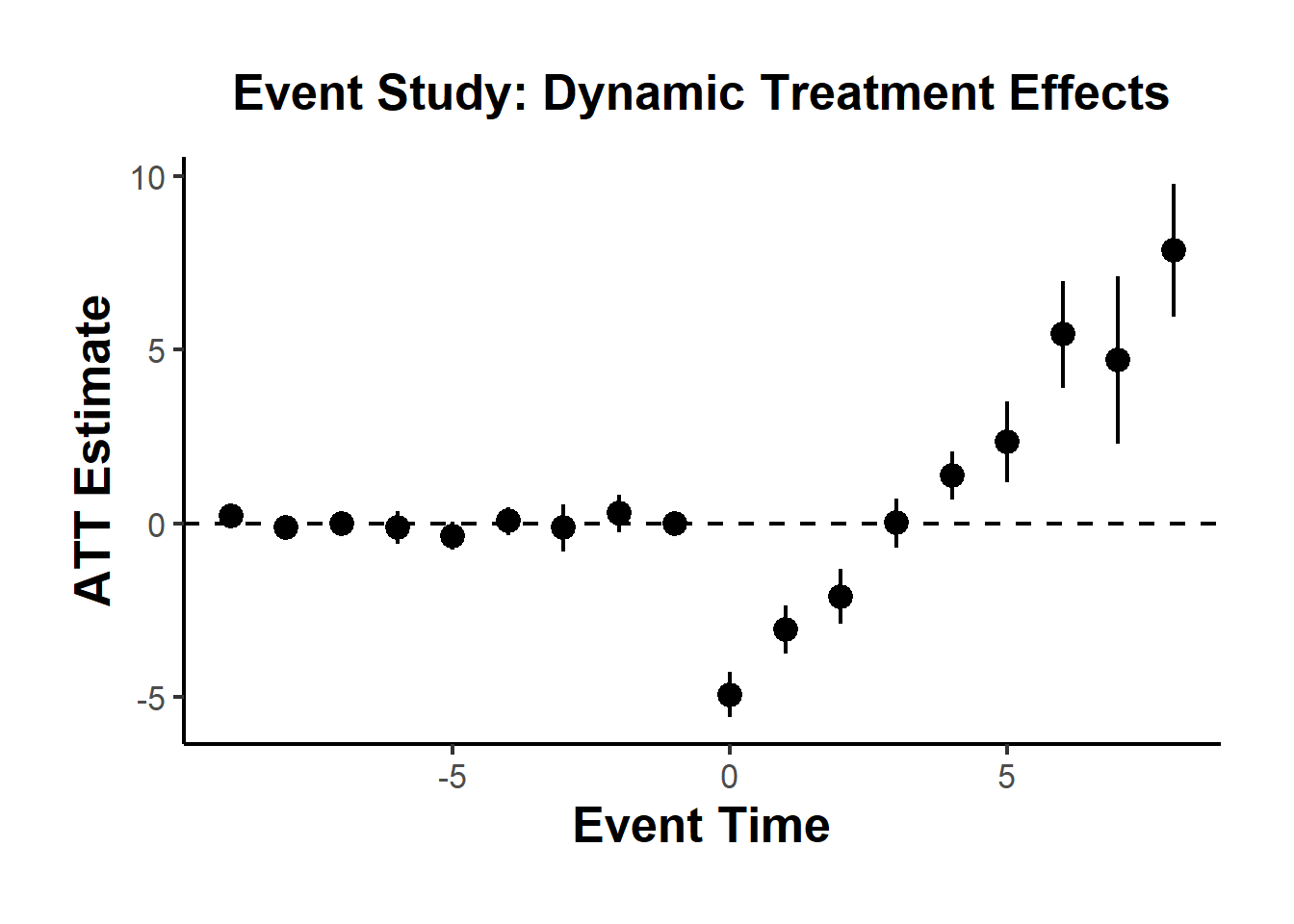

Figure 35.9: Event-study dynamic treatment effects.

The staggered package also includes direct implementations of alternative estimators:

• staggered_cs() implements the Callaway and Sant’Anna (2021) estimator.

• staggered_sa() implements the Sun and Abraham (2021) estimator, which adjusts for bias from comparisons involving already-treated units.

# Callaway and Sant’Anna estimator
staggered_cs(
    df = base_stagg,
    i = "id",
    t = "year",
    g = "year_treated",
    y = "y",
    estimand = "simple"
)
#>     estimate        se se_neyman
#> 1 -0.7994889 0.4484987 0.4486122

# Sun and Abraham estimator
staggered_sa(
    df = base_stagg,
    i = "id",
    t = "year",
    g = "year_treated",
    y = "y",
    estimand = "simple"
)
#>     estimate        se se_neyman
#> 1 -0.7551901 0.4407818 0.4409525

To assess statistical significance under the sharp null hypothesis \(H_0: \text{TE} = 0\), the staggered package includes an option for Fisher’s randomization (permutation) test. This approach tests whether the observed estimate could plausibly occur under a random reallocation of treatment timings.

# Fisher Randomization Test
staggered(
    df = base_stagg,
    i = "id",
    t = "year",
    g = "year_treated",
    y = "y",
    estimand = "simple",
    compute_fisher = TRUE,
    num_fisher_permutations = 100
)
#>     estimate        se se_neyman fisher_pval fisher_pval_se_neyman
#> 1 -0.7110941 0.2211943 0.2214245           0                     0
#>   num_fisher_permutations
#> 1                     100

This test provides a non-parametric method for inference and is particularly useful when the number of groups is small or standard errors are unreliable due to clustering or heteroskedasticity.

---

35.12.2 Cohort Average Treatment Effects (Sun and Abraham 2021)

Sun and Abraham (2021) propose a solution to the TWFE problem in staggered adoption settings by introducing an interaction-weighted estimator for dynamic treatment effects. This estimator is based on the concept of Cohort Average Treatment Effects on the Treated (CATT), which accounts for variation in treatment timing and dynamic treatment responses.

Traditional TWFE estimators implicitly assume homogeneous treatment effects and often rely on treated units serving as controls for later-treated units. When treatment effects vary over time or across groups, this leads to contaminated comparisons, especially in event-study specifications.

Sun and Abraham (2021) address this issue by:

• Estimating cohort-specific treatment effects relative to time since treatment.

• Using never-treated units as controls, or in their absence, the last-treated cohort.

35.12.2.1 Defining the Parameter of Interest: CATT

Let \(G_i = g\) denote the period when unit \(i\) first receives treatment. The cohort-specific average treatment effect on the treated (CATT) is defined as: \[ CATT_{g, l} = \mathbb{E}[Y_{i, g + l} - Y_{i, g + l}(0) \mid G_i = g] \] Where:

• \(l\) is the relative period (e.g., \(l = -1\) is one year before treatment, \(l = 0\) is the treatment year).

• \(Y_{i, g + l}(0)\) is the potential outcome without treatment.

• \(Y_{i, g + l}\) is the observed outcome.

This formulation allows one to trace out the dynamic effect of treatment for each cohort, relative to their treatment start time.

Sun and Abraham (2021) extend the interaction-weighted idea to panel settings, originally introduced by Gibbons et al. (2018) in a cross-sectional context.

They propose regressing the outcome on:

• Relative time indicators constructed by interacting treatment cohort (\(G_i\)) with time (\(t\)).

• Unit and time fixed effects.

This method explicitly estimates \(CATT_{g, l}\) terms, avoiding the contaminating influence of already-treated units that TWFE models often suffer from.

Relative Period Bin Indicator

\[ D_{it}^l = \mathbb{1}(t - G_i = l) \]

• \(G_i\): The time period when unit \(i\) first receives treatment.
• \(l\): The relative time period: how many periods have passed since treatment began.

1. Static Specification

\[ Y_{it} = \alpha_i + \lambda_t + \mu_g \sum_{l \ge 0} D_{it}^l + \epsilon_{it} \]

• \(\alpha_i\): Unit fixed effects.
• \(\lambda_t\): Time fixed effects.
• \(\mu_g\): Effect for group \(g\).
• Excludes periods prior to treatment.

2. Dynamic Specification

\[ Y_{it} = \alpha_i + \lambda_t + \sum_{\substack{l = -K \\ l \neq -1}}^{L} \mu_l D_{it}^l + \epsilon_{it} \]

• Includes leads and lags of treatment indicators \(D_{it}^l\).
• Excludes one period (typically \(l = -1\)) to avoid perfect collinearity.
• Tests for pre-treatment parallel trends rely on the leads (\(l < 0\)).

---

35.12.2.2 Identifying Assumptions

1. Parallel Trends

For identification, it is assumed that untreated potential outcomes follow parallel trends across cohorts in the absence of treatment: \[ \mathbb{E}[Y_{it}(0) - Y_{i, t-1}(0) \mid G_i = g] = \text{constant across } g \] This allows us to use never-treated or not-yet-treated units as valid counterfactuals.

2. No Anticipatory Effects

Treatment should not influence outcomes before it is implemented. That is: \[ CATT_{g, l} = 0 \quad \text{for all } l < 0 \] This ensures that any pre-trends are not driven by behavioral changes in anticipation of treatment.

3. Treatment Effect Homogeneity (Optional)

The treatment effect is consistent across cohorts for each relative period. Each adoption cohort should have the same path of treatment effects. In other words, the trajectory of each treatment cohort is similar.

Although Sun and Abraham (2021) allow treatment effect heterogeneity, some settings may assume homogeneous effects within cohorts and periods:

• Each cohort has the same pattern of response over time.

• This is relaxed in their design but assumed in simpler TWFE settings.

35.12.2.3 Comparison to Other Designs

Different DiD designs make distinct assumptions about how treatment effects vary (Table 35.7)

Table 35.7: Comparison of designs’ assumptions.

Study	Vary Over Time	Vary Across Cohorts	Notes
Sun and Abraham (2021)	✓	✓	Allows full heterogeneity
Callaway and Sant’Anna (2021)	✓	✓	Estimates group × time ATTs
Borusyak et al. (2024)	✓	✗	Homogeneous across cohorts Heterogeneity over time
Athey and Imbens (2022)	✗	✓	Heterogeneity only across adoption cohorts
De Chaisemartin and D’haultfœuille (2023)	✓	✓	Complete heterogeneity
Goodman-Bacon (2021)	✓ or ✗	✗ or ✓	Restricts one dimension Heterogeneity either “vary across units but not over time” or “vary over time but not across units”.

35.12.2.4 Sources of Treatment Effect Heterogeneity

Several forces can generate heterogeneous treatment effects:

• Calendar Time Effects: macro events (e.g., recessions, policy changes) affect cohorts differently.

• Selection into Timing: units self-select into early/late treatment based on anticipated effects.

• Composition Differences: adoption cohorts may differ in observed or unobserved ways.

Such heterogeneity can bias TWFE estimates, which often average effects across incomparable groups.

---

35.12.2.5 Technical Issues

When using an event-study TWFE regression to estimate dynamic treatment effects in staggered adoption settings, one must exclude certain relative time indicators to avoid perfect multicollinearity. This arises because relative period indicators are linearly dependent due to the presence of unit and time fixed effects.

Specifically, the following two terms must be addressed:

• The period immediately before treatment (\(l = -1\)): this period is typically omitted and serves as the baseline for comparison. This normalization has been standard practice in event study regressions prior to Sun and Abraham (2021) .

• A distant post-treatment period (e.g., \(l = +5\) or \(l = +10\)): Sun and Abraham (2021) clarified that in addition to the baseline period, at least one other relative time indicator, typically from the far tail of the post-treatment distribution, must be dropped, binned, or trimmed to avoid multicollinearity among the relative time dummies. This issue emerges because fixed effects absorb much of the within-unit and within-time variation, reducing the effective rank of the design matrix.

Dropping certain relative periods (especially pre-treatment periods) introduces an implicit normalization: the estimates for included periods are now interpreted relative to the omitted periods. If treatment effects are present in these omitted periods (e.g., due to anticipation or early effects), this will contaminate the estimates of included relative periods.

To avoid this contamination, researchers often assume that all pre-treatment periods have zero treatment effect, i.e.,

\[ CATT_{g, l} = 0 \quad \text{for all } l < 0 \]

This assumption ensures that excluded pre-treatment periods form a valid counterfactual, and estimates for \(l \geq 0\) are not biased due to normalization.

---

Sun and Abraham (2021) resolve the issues of weighting and aggregation by using a clean weighting scheme that avoids contamination from excluded periods. Their method produces a weighted average of cohort- and time-specific treatment effects (\(CATT_{g, l}\)), where the weights are:

• Non-negative
• Sum to one
• Interpretable as the fraction of treated units who are observed \(l\) periods after treatment, normalized over the number of available periods \(g\)

This interaction-weighted estimator ensures that the estimated average treatment effect reflects a convex combination of dynamic treatment effects from different cohorts and times.

In this way, their aggregation logic closely mirrors that of Callaway and Sant’Anna (2021), who also construct average treatment effects from group-time ATTs using interpretable weights that align with the sampling structure.

---

library(fixest)
data("base_stagg")

# Estimate Sun & Abraham interaction-weighted model
res_sa20 <- feols(
  y ~ x1 + sunab(year_treated, year) | id + year,
  data = base_stagg
)

Use iplot() to visualize the estimated dynamic treatment effects across relative time (Figure 35.10)

iplot(res_sa20)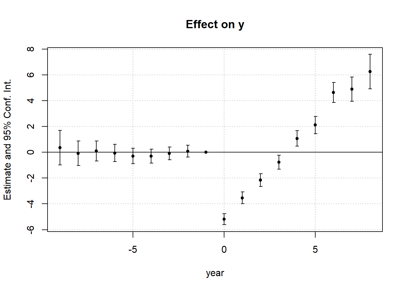

Figure 35.10: Estimated dynamic treatment effects on \(y\) across relative time.

You can summarize the results using different aggregation options:

# Overall average ATT
summary(res_sa20, agg = "att")
#> OLS estimation, Dep. Var.: y
#> Observations: 950
#> Fixed-effects: id: 95,  year: 10
#> Standard-errors: IID 
#>      Estimate Std. Error  t value   Pr(>|t|)    
#> x1   0.994678   0.018823 52.84242  < 2.2e-16 ***
#> ATT -1.133749   0.194764 -5.82113 8.6022e-09 ***
#> ---
#> Signif. codes:  0 '***' 0.001 '**' 0.01 '*' 0.05 '.' 0.1 ' ' 1
#> RMSE: 0.921817     Adj. R2: 0.887984
#>                  Within R2: 0.876406

# Aggregation across post-treatment periods (excluding leads)
summary(res_sa20, agg = c("att" = "year::[^-]"))
#> OLS estimation, Dep. Var.: y
#> Observations: 950
#> Fixed-effects: id: 95,  year: 10
#> Standard-errors: IID 
#>                      Estimate Std. Error   t value   Pr(>|t|)    
#> x1                   0.994678   0.018823 52.842416  < 2.2e-16 ***
#> year::-9:cohort::10  0.351766   0.682887  0.515116 6.0662e-01    
#> year::-8:cohort::9   0.033914   0.682561  0.049686 9.6039e-01    
#> year::-8:cohort::10 -0.191932   0.681848 -0.281488 7.7841e-01    
#> year::-7:cohort::8  -0.589387   0.681850 -0.864394 3.8764e-01    
#> year::-7:cohort::9   0.872995   0.683597  1.277061 2.0197e-01    
#> year::-7:cohort::10  0.019512   0.682179  0.028603 9.7719e-01    
#> year::-6:cohort::7  -0.042147   0.681865 -0.061811 9.5073e-01    
#> year::-6:cohort::8  -0.657571   0.682009 -0.964167 3.3527e-01    
#> year::-6:cohort::9   0.877743   0.682578  1.285923 1.9886e-01    
#> year::-6:cohort::10 -0.403635   0.681921 -0.591909 5.5409e-01    
#> year::-5:cohort::6  -0.658034   0.682137 -0.964666 3.3502e-01    
#> year::-5:cohort::7  -0.316974   0.683243 -0.463926 6.4283e-01    
#> year::-5:cohort::8  -0.238213   0.682050 -0.349261 7.2699e-01    
#> year::-5:cohort::9   0.301477   0.684068  0.440712 6.5955e-01    
#> year::-5:cohort::10 -0.564801   0.681846 -0.828340 4.0774e-01    
#> year::-4:cohort::5  -0.983453   0.681867 -1.442295 1.4963e-01    
#> year::-4:cohort::6   0.360407   0.682386  0.528156 5.9754e-01    
#> year::-4:cohort::7  -0.430610   0.681846 -0.631535 5.2788e-01    
#> year::-4:cohort::8  -0.895195   0.681846 -1.312898 1.8961e-01    
#> year::-4:cohort::9  -0.392478   0.682433 -0.575116 5.6538e-01    
#> year::-4:cohort::10  0.519001   0.681901  0.761110 4.4683e-01    
#> year::-3:cohort::4   0.591288   0.681879  0.867144 3.8614e-01    
#> year::-3:cohort::5  -1.000650   0.682072 -1.467074 1.4277e-01    
#> year::-3:cohort::6   0.072188   0.681865  0.105868 9.1571e-01    
#> year::-3:cohort::7  -0.836820   0.681850 -1.227279 2.2010e-01    
#> year::-3:cohort::8  -0.783148   0.681958 -1.148382 2.5117e-01    
#> year::-3:cohort::9   0.811285   0.682635  1.188461 2.3502e-01    
#> year::-3:cohort::10  0.527203   0.682593  0.772354 4.4014e-01    
#> year::-2:cohort::3   0.036941   0.682296  0.054143 9.5684e-01    
#> year::-2:cohort::4   0.832250   0.681851  1.220575 2.2262e-01    
#> year::-2:cohort::5  -1.574086   0.681930 -2.308281 2.1250e-02 *  
#> year::-2:cohort::6   0.311758   0.681848  0.457225 6.4764e-01    
#> year::-2:cohort::7  -0.558631   0.681891 -0.819239 4.1291e-01    
#> year::-2:cohort::8   0.429591   0.681861  0.630028 5.2886e-01    
#> year::-2:cohort::9   1.201899   0.681871  1.762649 7.8359e-02 .  
#> year::-2:cohort::10 -0.002429   0.682085 -0.003562 9.9716e-01    
#> att                 -1.133749   0.194764 -5.821130 8.6022e-09 ***
#> ---
#> Signif. codes:  0 '***' 0.001 '**' 0.01 '*' 0.05 '.' 0.1 ' ' 1
#> RMSE: 0.921817     Adj. R2: 0.887984
#>                  Within R2: 0.876406

# Aggregate post-treatment effects from l = 0 to 8
summary(res_sa20, agg = c("att" = "year::[012345678]")) |> 
  etable(digits = 2)
#>                         summary(res_..
#> Dependent Var.:                      y
#>                                       
#> x1                      0.99*** (0.02)
#> year = -9 x cohort = 10    0.35 (0.68)
#> year = -8 x cohort = 9     0.03 (0.68)
#> year = -8 x cohort = 10   -0.19 (0.68)
#> year = -7 x cohort = 8    -0.59 (0.68)
#> year = -7 x cohort = 9     0.87 (0.68)
#> year = -7 x cohort = 10    0.02 (0.68)
#> year = -6 x cohort = 7    -0.04 (0.68)
#> year = -6 x cohort = 8    -0.66 (0.68)
#> year = -6 x cohort = 9     0.88 (0.68)
#> year = -6 x cohort = 10   -0.40 (0.68)
#> year = -5 x cohort = 6    -0.66 (0.68)
#> year = -5 x cohort = 7    -0.32 (0.68)
#> year = -5 x cohort = 8    -0.24 (0.68)
#> year = -5 x cohort = 9     0.30 (0.68)
#> year = -5 x cohort = 10   -0.56 (0.68)
#> year = -4 x cohort = 5    -0.98 (0.68)
#> year = -4 x cohort = 6     0.36 (0.68)
#> year = -4 x cohort = 7    -0.43 (0.68)
#> year = -4 x cohort = 8    -0.90 (0.68)
#> year = -4 x cohort = 9    -0.39 (0.68)
#> year = -4 x cohort = 10    0.52 (0.68)
#> year = -3 x cohort = 4     0.59 (0.68)
#> year = -3 x cohort = 5     -1.0 (0.68)
#> year = -3 x cohort = 6     0.07 (0.68)
#> year = -3 x cohort = 7    -0.84 (0.68)
#> year = -3 x cohort = 8    -0.78 (0.68)
#> year = -3 x cohort = 9     0.81 (0.68)
#> year = -3 x cohort = 10    0.53 (0.68)
#> year = -2 x cohort = 3     0.04 (0.68)
#> year = -2 x cohort = 4     0.83 (0.68)
#> year = -2 x cohort = 5    -1.6* (0.68)
#> year = -2 x cohort = 6     0.31 (0.68)
#> year = -2 x cohort = 7    -0.56 (0.68)
#> year = -2 x cohort = 8     0.43 (0.68)
#> year = -2 x cohort = 9     1.2. (0.68)
#> year = -2 x cohort = 10  -0.002 (0.68)
#> att                     -1.1*** (0.19)
#> Fixed-Effects:          --------------
#> id                                 Yes
#> year                               Yes
#> _______________________ ______________
#> S.E. type                          IID
#> Observations                       950
#> R2                             0.90982
#> Within R2                      0.87641
#> ---
#> Signif. codes: 0 '***' 0.001 '**' 0.01 '*' 0.05 '.' 0.1 ' ' 1

The fwlplot package provides diagnostics for how much variation is explained by fixed effects or covariates (Figures 35.11, 35.12 and 35.13).

library(fwlplot)

# Simple FWL plot
fwl_plot(y ~ x1, data = base_stagg)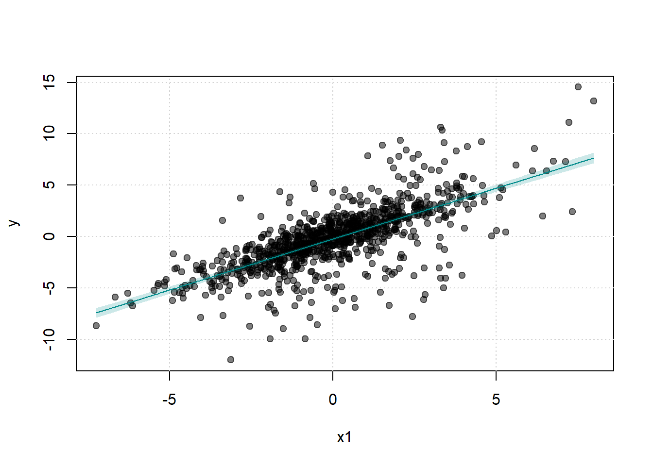

Figure 35.11: Scatter plot of \(y\) against \(x_1\).

# With fixed effects
fwl_plot(y ~ x1 | id + year,
         data = base_stagg,
         n_sample = 100)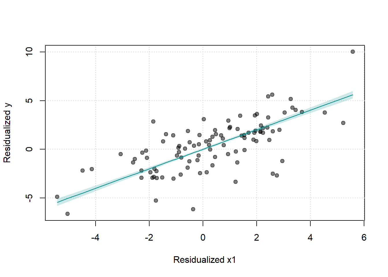

Figure 35.12: Scatter plot of residualized \(y\) against residualized \(x_1\).

# Splitting by treatment status
fwl_plot(
    y ~ x1 |
        id + year,
    data = base_stagg,
    n_sample = 100,
    fsplit = ~ treated
)

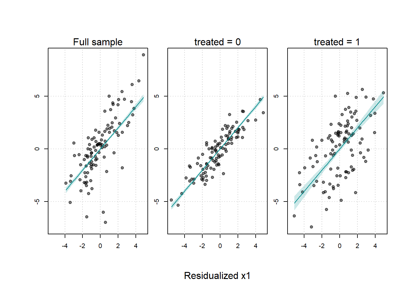
Figure 35.13: Scatter plot of residualized \(y\) against residualized \(x_1\) by treatment status.

---

35.12.3 Stacked Difference-in-Differences

The Stacked DiD approach addresses key limitations of standard TWFE models in staggered adoption designs, particularly treatment effect heterogeneity and timing variations. By constructing sub-experiments around each treatment event, researchers can isolate cleaner comparisons and reduce contamination from improperly specified control groups.

Basic TWFE Specification

\[ Y_{it} = \beta_{FE} D_{it} + A_i + B_t + \epsilon_{it} \]

• \(Y_{it}\): Outcome for unit \(i\) at time \(t\).
• \(D_{it}\): Treatment indicator (1 if treated, 0 otherwise).
• \(A_i\): Unit (group) fixed effects.
• \(B_t\): Time period fixed effects.
• \(\epsilon_{it}\): Idiosyncratic error term.

---

Steps in the Stacked DiD Procedure

35.12.3.1 Choose an Event Window

Define:

• \(\kappa_a\): number of pre-treatment periods to include in the event window (lead periods).
• \(\kappa_b\): number of post-treatment periods to include in the event window (lag periods).

Implication:
Only events where sufficient pre- and post-treatment periods exist will be included (i.e., excluding those events that do not meet this criteria).

---

35.12.3.2 Enumerate Sub-Experiments

Define:

• \(T_1\): First period in the panel.
• \(T_T\): Last period in the panel.
• \(\Omega_A\): The set of treatment adoption periods that fit within the event window:

\[ \Omega_A = \left\{ A_i \middle| T_1 + \kappa_a \le A_i \le T_T - \kappa_b \right\} \]

• Each \(A_i\) represents an adoption period for unit \(i\) that has enough time on both sides of the event.

Let \(d = 1, \dots, D\) index the sub-experiments in \(\Omega_A\).

• \(\omega_d\): The event (adoption) date of the \(d\)-th sub-experiment.

---

35.12.3.3 Define Inclusion Criteria

Valid Treated Units

• In sub-experiment \(d\), treated units have adoption date exactly equal to \(\omega_d\).
• A unit may only be treated in one sub-experiment to avoid duplication.

Clean Control Units

• Controls are units where \(A_i > \omega_d + \kappa_b\), i.e.,
  • They are never treated, or
  • They are treated in the far future (beyond the post-event window).
• A control unit can appear in multiple sub-experiments, but this requires correcting standard errors (see below).

Valid Time Periods

• Only observations where
  \[ \omega_d - \kappa_a \le t \le \omega_d + \kappa_b \]
  are included.
• This ensures the analysis is centered on the event window.

35.12.3.4 Specify Estimating Equation

Basic DiD Specification in the Stacked Dataset

\[ Y_{itd} = \beta_0 + \beta_1 T_{id} + \beta_2 P_{td} + \beta_3 (T_{id} \times P_{td}) + \epsilon_{itd} \]

Where:

• \(i\): Unit index

• \(t\): Time index

• \(d\): Sub-experiment index

• \(T_{id}\): Indicator for treated units in sub-experiment \(d\)

• \(P_{td}\): Indicator for post-treatment periods in sub-experiment \(d\)

• \(\beta_3\): Captures the DiD estimate of the treatment effect.

Equivalent Form with Fixed Effects

\[ Y_{itd} = \beta_3 (T_{id} \times P_{td}) + \theta_{id} + \gamma_{td} + \epsilon_{itd} \]

where

• \(\theta_{id}\): Unit-by-sub-experiment fixed effect.

• \(\gamma_{td}\): Time-by-sub-experiment fixed effect.

Note:

• \(\beta_3\) summarizes the average treatment effect across all sub-experiments but does not allow for dynamic effects by time since treatment.

35.12.3.5 Stacked Event Study Specification

Define Time Since Event (\(YSE_{td}\)):

\[ YSE_{td} = t- \omega_d \]

where

• Measures time since the event (relative time) in sub-experiment \(d\).

• \(YSE_{td} \in [-\kappa_a, \dots, 0, \dots, \kappa_b]\) in every sub-experiment.

Event-Study Regression (Sub-Experiment Level)

\[ Y_{it}^d = \sum_{j = -\kappa_a}^{\kappa_b} \beta_j^d . 1 (YSE_{td} = j) + \sum_{j = -\kappa_a}^{\kappa_b} \delta_j^d (T_{id} . 1 (YSE_{td} = j)) + \theta_i^d + \epsilon_{it}^d \]

where

• Separate coefficients for each sub-experiment \(d\).

• \(\delta_j^d\): Captures treatment effects at relative time \(j\) within sub-experiment \(d\).

Pooled Stacked Event-Study Regression

\[ Y_{itd} = \sum_{j = -\kappa_a}^{\kappa_b} \beta_j \cdot \mathbb{1}(YSE_{td} = j) + \sum_{j = -\kappa_a}^{\kappa_b} \delta_j \left( T_{id} \cdot \mathbb{1}(YSE_{td} = j) \right) + \theta_{id} + \epsilon_{itd} \]

• Pooled coefficients \(\delta_j\) reflect average treatment effects by event time \(j\) across sub-experiments.

35.12.3.6 Clustering in Stacked DID

• Cluster at Unit by Sub-Experiment Level (Cengiz et al. 2019): accounts for units appearing multiple times across sub-experiments.

• Cluster at Unit Level (Deshpande and Li 2019): appropriate when units are uniquely identified and do not appear in multiple sub-experiments.

---

library(did)
library(tidyverse)
library(fixest)

# Load example data
data(base_stagg)

# Get treated cohorts (exclude never-treated units coded as 10000)
cohorts <- base_stagg %>%
    filter(year_treated != 10000) %>%
    distinct(year_treated) %>%
    pull()

# Function to generate data for each sub-experiment
getdata <- function(j, window) {
    base_stagg %>%
        filter(
            year_treated == j |               # treated units in cohort j
            year_treated > j + window         # controls not treated soon after
        ) %>%
        filter(
            year >= j - window &
            year <= j + window                # event window bounds
        ) %>%
        mutate(df = j)                        # sub-experiment indicator
}

# Generate the stacked dataset
stacked_data <- map_df(cohorts, ~ getdata(., window = 5)) %>%
    mutate(
        rel_year = if_else(df == year_treated, time_to_treatment, NA_real_)
    ) %>%
    fastDummies::dummy_cols("rel_year", ignore_na = TRUE) %>%
    mutate(across(starts_with("rel_year_"), ~ replace_na(., 0)))

# Estimate fixed effects regression on the stacked data
stacked_result <- feols(
    y ~ `rel_year_-5` + `rel_year_-4` + `rel_year_-3` + `rel_year_-2` +
        rel_year_0 + rel_year_1 + rel_year_2 + rel_year_3 +
        rel_year_4 + rel_year_5 |
        id ^ df + year ^ df,
    data = stacked_data
)

# Extract coefficients and standard errors
stacked_coeffs <- stacked_result$coefficients
stacked_se <- stacked_result$se

# Insert zero for the omitted period (usually -1)
stacked_coeffs <- c(stacked_coeffs[1:4], 0, stacked_coeffs[5:10])
stacked_se <- c(stacked_se[1:4], 0, stacked_se[5:10])

# Plotting estimates from three methods: Callaway & Sant'Anna, Sun & Abraham, and Stacked DiD

cs_out <- att_gt(
    yname = "y",
    data = base_stagg,
    gname = "year_treated",
    idname = "id",
    # xformla = "~x1",
    tname = "year"
)
cs <-
    aggte(
        cs_out,
        type = "dynamic",
        min_e = -5,
        max_e = 5,
        bstrap = FALSE,
        cband = FALSE
    )



res_sa20 = feols(y ~ sunab(year_treated, year) |
                     id + year, base_stagg)
sa = tidy(res_sa20)[5:14, ] %>% pull(estimate)
sa = c(sa[1:4], 0, sa[5:10])

sa_se = tidy(res_sa20)[6:15, ] %>% pull(std.error)
sa_se = c(sa_se[1:4], 0, sa_se[5:10])

compare_df_est = data.frame(
    period = -5:5,
    cs = cs$att.egt,
    sa = sa,
    stacked = stacked_coeffs
)

compare_df_se = data.frame(
    period = -5:5,
    cs = cs$se.egt,
    sa = sa_se,
    stacked = stacked_se
)

compare_df_longer <- compare_df_est %>%
    pivot_longer(!period, names_to = "estimator", values_to = "est") %>%
    full_join(compare_df_se %>%
                  pivot_longer(!period, names_to = "estimator", values_to = "se")) %>%
    mutate(upper = est +  1.96 * se,
           lower = est - 1.96 * se)

Figure 35.14 shows a comparison between three estimators (i.e., CS, SA, and stacked)

ggplot(compare_df_longer) +
    geom_ribbon(aes(
        x = period,
        ymin = lower,
        ymax = upper,
        group = estimator
    ), alpha = 0.2) +
    geom_line(aes(
        x = period,
        y = est,
        group = estimator,
        color = estimator
    ),
    linewidth = 1.2) +
    
    labs(
        title = "Comparison of Dynamic Treatment Effects",
        x = "Event Time (Periods since Treatment)",
        y = "Estimated ATT",
        color = "Estimator"
    ) + 
    causalverse::ama_theme()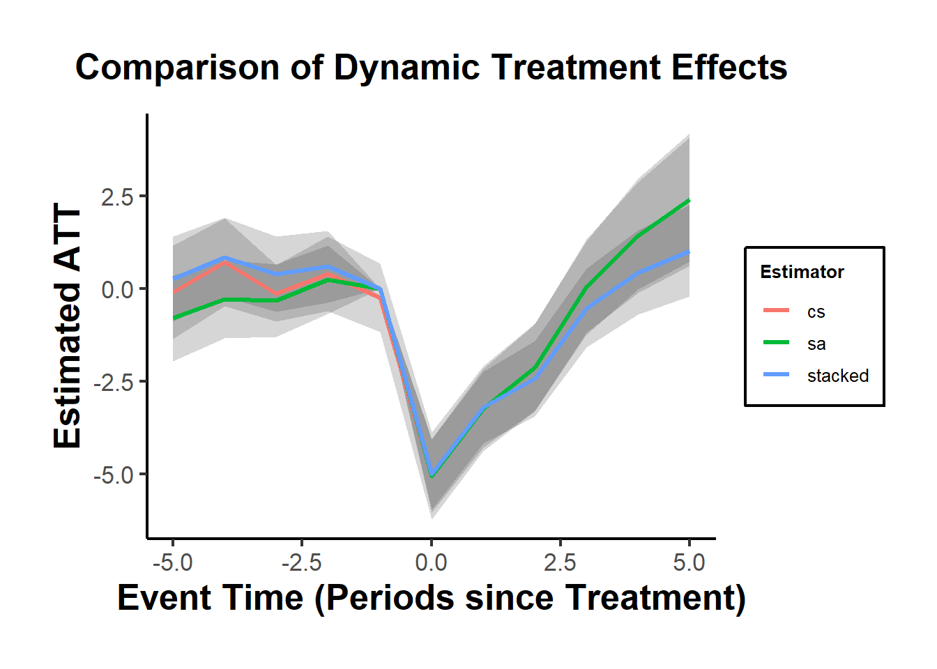

Figure 35.14: Comparison of dynamic average treatment effects across CS, SA, and stacked estimators.

---

35.12.4 Panel Match DiD Estimator with In-and-Out Treatment Conditions

The Panel Match estimator is the natural choice when treatment is genuinely a switch rather than an absorbing event: countries democratize and then revert, firms adopt and later abandon a marketing channel, regulators turn a policy on and then off. Estimators built for staggered adoption, such as the cohort approach in Section 35.12.2 and the group-time framework in Section 35.12.1, assume treatment is monotone (once on, always on), an assumption that quietly fails in many political-economy and managerial panels. Panel Match relaxes monotonicity, accommodates carryover, and replaces functional-form discipline with explicit matching on treatment history. The cost, as we will see, is statistical efficiency and analyst effort: matched sets shrink quickly as the lag window grows, so every assumption relaxed has to be paid for in variance.

As noted in Imai and Kim (2021), the TWFE regression model is widely used but fundamentally relies on strong modeling assumptions, particularly linearity and additivity. It does not constitute a fully nonparametric estimation method and may yield biased results under model misspecification. Section 35.13 catalogues the failure modes that motivate a design-based alternative.

Researchers often prefer TWFE due to its ability to control for both unit- and time-specific unobserved confounders:

• \(\alpha_i = h(\mathbf{U}_i)\) accounts for unit-level confounders.
• \(\gamma_t = f(\mathbf{V}_t)\) adjusts for time-level confounders.

The functional forms \(h(\cdot)\) and \(f(\cdot)\) are left unspecified, but additivity and separability are assumed. TWFE is based on the model:

\[ Y_{it} = \alpha_i + \gamma_t + \beta X_{it} + \epsilon_{it} \]

for \(i = 1, \dots, N\), and \(t = 1, \dots, T\). However, this formulation requires a linear specification for the treatment effect \(\beta\). Contrary to popular belief, the model does require functional form assumptions for validity (Imai and Kim 2021, 406; 2019).

---

35.12.4.1 Matching and the Panel Match DiD Estimator

To mitigate model dependence and improve causal inference validity, Imai and Kim (2021) propose a matching-based framework for panel data. This method is implemented via the wfe and PanelMatch R packages and offers design-based identification (Section 31.7.1) under relaxed assumptions. Conceptually, Panel Match takes the logic of cross-sectional matching and lifts it into time, treating each treated unit-period as a small case study with its own bespoke control group.

This setting generalizes staggered adoption, allowing units to transition in and out of treatment. The core idea is to construct matched control groups that share the same treatment history as treated units and then apply a Difference-in-Differences logic. This is better than synthetic controls (e.g., Xu (2017)) because it requires less data to achieve good performance and can adapt to contexts where units switch treatment status multiple times. Compared with the synthetic DiD and matrix completion approaches, Panel Match trades a global low-rank model of the outcome for local matched comparisons, an attractive bargain when the analyst trusts treatment-history matching but is uncomfortable specifying a factor structure.

Key Properties of PM-DiD (Imai, Kim, et al. 2021)

• Designed for multiple treatment switches over time.
• Addresses issues of carryover, reversal, and attenuation bias.
• Allows estimation of short-term and long-term causal effects, accounting for time dynamics.

Key Findings (Imai, Kim, et al. 2021)

• Even under favorable conditions for OLS, PM-DiD is more robust to model misspecification and omitted lags.

• This robustness comes with a cost: reduced efficiency (larger variance).

• Reflects the classic bias-variance tradeoff between flexible and parametric estimators.

Data and Software Requirements

• Treatment variable: binary (0 = control, 1 = treated).

• Unit and time variables: integer/numeric and ordered.

• Input data must be in data.frame format.

The method is well suited to long-running political-economy panels in which units repeatedly enter and exit treatment regimes. Scheve and Stasavage (2012)’s study of democratization and its effect on top-income taxation, and Acemoglu et al. (2019)’s panel analysis of democracy and economic growth, are two influential examples of exactly this structure: a binary treatment switching on and off across countries over a long horizon, with a research question that demands a credible counterfactual for each treated country at each treated moment.

In choosing among modern estimators surveyed in Section 35.12, the practical question is rarely “which is correct?” but rather “which assumptions are tolerable in this dataset?” Panel Match dominates the alternatives when several conditions co-occur: the treatment switches on and off, the analyst suspects nonlinear or nonadditive confounding, and the panel is long enough that requiring identical histories over \(L\) lags still leaves a workable matched set. When treatment is monotone and cohorts are well populated, the Callaway and Sant’Anna group-time estimator or Sun and Abraham cohort estimator typically deliver tighter inference. When matching across unit-time pairs is too thin to support a credible matched set, counterfactual estimators such as the matrix completion approach in Section 35.12.6 borrow strength from the full control panel and may be preferable. In short, Panel Match is the right tool for treatment patterns that other estimators were not built to accommodate, but the price is paid in efficiency and in a heavier diagnostic burden.

---

35.12.4.2 Two-Way Matching Interpretation of TWFE

Before introducing Panel Match’s matched sets, it helps to see exactly what TWFE is already doing under the hood. Reframing TWFE as an implicit matching estimator clarifies both why it works in textbook two-period settings and why it goes off the rails in the staggered, switching designs that motivate Panel Match. The Goodman-Bacon decomposition (Section 35.6.3.1) tells the same story in the language of weighted DiD comparisons.

The least squares estimate of \(\beta\) in the TWFE model can be re-expressed as a matching estimator that compares each treated unit to observations within:

• The same unit (within-unit match),
• The same time period (within-time match),
• Adjusted by a third set of observations in neither group.

This leads to mismatches: treated observations compared to units with the same treatment status, which causes attenuation bias.

The adjustment factor \(K\) corrects for this by weighting matches appropriately. However, even the weighted TWFE estimator contains some mismatches and relies on comparisons across units that differ in key characteristics.

In the simple two-period, two-group DiD setting, the TWFE and DiD estimators coincide. However, in multi-period DiD with treatment reversals, this equivalence breaks down (Imai and Kim 2021).

• The unweighted TWFE is not equivalent to multi-period DiD.
• The multi-period DiD is equivalent to a weighted TWFE, but some weights are negative, which is a problematic feature from a design-based perspective.

This means that justifying TWFE via DiD logic is incorrect unless the linearity assumption is satisfied. The same warning surfaces in the broader literature on negative weighting: see the switching DiD discussion and the reshaped IPW construction below.

---

35.12.4.3 Estimation Using Panel Match DiD

The estimation procedure can be read as a sequence of four conceptual moves. First, restrict attention to units whose recent past resembles the treated unit, so that any remaining outcome difference cannot plausibly be attributed to an earlier treatment. Second, refine within that history-matched pool using the standard cross-sectional matching toolkit so that observable covariates also balance. Third, run the simplest possible DiD on the resulting pair to read off the post-treatment effect. Fourth, audit the construction by examining whether covariates are in fact balanced after refinement. Each step echoes a familiar move from the matching literature, but the discipline of also matching on treatment history is what carries the design through staggered onset and treatment reversal.

Core Estimation Steps (Imai, Kim, et al. 2021):

1. Match treated observations with control observations from the same time period and with identical treatment histories over the past \(L\) periods.
2. Use standard matching or weighting methods to refine control sets (e.g., Mahalanobis distance, propensity score).
3. Apply a DiD estimator to compute treatment effects at time \(t + F\).
4. Evaluate match quality using covariate balance diagnostics (Ho et al. 2007).

Causal Estimand

Let \(F\) be the number of leads (future periods) and \(L\) be the number of lags (past treatment periods). Define the average treatment effect as:

\[ \delta(F, L) = \mathbb{E}\left[Y_{i, t+F}(1) - Y_{i, t+F}(0) \mid \text{treatment history from } t-L \text{ to } t\right] \]

• \(F = 0\): contemporaneous effect (short-run ATT)
• \(F > 0\): future outcomes (long-run ATT)
• \(L\): adjusts for potential carryover effects

The estimator also allows for estimation of the Average Reversal Treatment Effect (ART) when treatment status switches from 1 to 0.

---

35.12.4.4 Model Assumptions

The assumption ledger looks lighter than TWFE’s, but each item carries a practical cost:

• No spillover effects across units (i.e., SUTVA holds). When the units of analysis are countries or large markets, this assumption is rarely innocuous and has to be defended substantively.

• Carryover effects allowed up to \(L\) periods. The analyst must specify how long the past of treatment is allowed to matter; this transfers a modeling decision into a window choice.

• After \(L\) lags, prior treatments are assumed to have no effect on \(Y_{i,t+F}\). Persistent treatment dynamics that exceed the chosen window are forced to live inside the residual.

• The potential outcome at \(t + F\) is independent of treatment assignments beyond \(t - L\). This is the formal restriction that lets the analyst stop at \(L\).

• The key identifying assumption is a conditional parallel trends assumption. Outcome trends are assumed parallel across treated and matched control units, conditional on:

  • Past treatment,

  • Covariate histories,

  • Lagged outcomes (excluding the most recent).

  Unlike standard TWFE, strong ignorability (Section 31.5.2) is not required, and the overlap requirement is satisfied automatically by the matched-set construction whenever a match exists.

The cost of trading parametric structure for matching is straightforward but easily underestimated. Each additional lag in \(L\) multiplies the number of distinct treatment histories that must be matched exactly, so matched sets shrink geometrically with the lag window. In the empirical illustrations below, a four-year history requirement already eliminates a sizeable share of treated observations from the analysis. Carryover and parallel-trends violations beyond the chosen \(L\) are absorbed silently into the estimator. In return, the analyst is freed from the linearity and additivity assumptions that drive TWFE bias under heterogeneous effects.

---

35.12.4.5 Covariate Balance Assessment

Balance diagnostics earn their keep here in a way they do not in cross-sectional matching, because they are the principal evidence that the conditional parallel-trends assumption is plausible. Where regression-based DiD asks the reader to trust the parametric model, Panel Match exposes the comparison directly. The diagnostics are therefore not a final cosmetic check but a first-class identification argument.

Assessing balance before estimating ATT is critical:

• Compute the mean standardized difference between treated and matched control units.
• Check balance across covariates and lagged outcomes for all \(L\) pretreatment periods.
• Imbalanced covariates may indicate violations of the parallel trends assumption; the same diagnostic logic underpins the placebo tests and the broader robustness checks used in quasi-experimental work.

---

35.12.4.6 Implementing the Panel Match DiD Estimator

library(PanelMatch)

Treatment Variation Plot

Visualizing the variation of treatment across space and time is essential to assess whether the treatment has sufficient heterogeneity to support credible causal identification (Figure 35.15).

DisplayTreatment(
  panel.data = PanelData(
    panel.data = dem,
    unit.id = "wbcode2",
    time.id = "year",
    treatment = "dem",
    outcome = "y"
  ),
  legend.position = "none",
  xlab = "year",
  ylab = "Country Code"
)

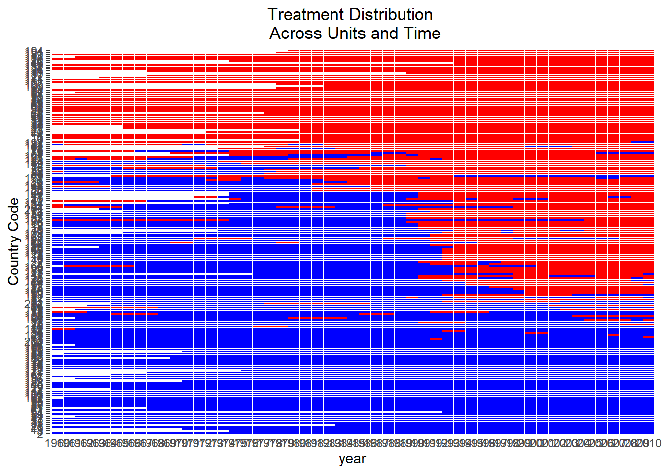
Figure 35.15: Treatment distribution across units and time.

• This plot aids in identifying whether the treatment is broadly distributed or concentrated among a few units or time periods.

• Insufficient treatment variation may weaken identification or reduce the precision of estimated effects.

35.12.4.6.1 Setting Parameters \(F\) and \(L\)

The two tuning parameters \(F\) and \(L\) encode the substantive question. \(F\) asks how far after treatment the analyst wants to look, which is a question about post-treatment dynamics. \(L\) asks how much of the past should be allowed to differ between treated and control units before the comparison becomes uninterpretable, which is a question about pretreatment confounding. In practice analysts try several pairs and report results under each, the same sensitivity philosophy used elsewhere in the robustness checks literature.

1. Select \(F\): the number of leads, or time periods after treatment, for which the effect is measured.

• \(F = 0\): contemporaneous (short-term) treatment effect.

• \(F > 0\): long-term or cumulative effects.

2. Select \(L\): the number of lags (prior treatment periods) used in matching to adjust for carryover effects.

• Increasing \(L\) enhances credibility but reduces match quality and sample size.

• This selection reflects the bias-variance tradeoff.

---

35.12.4.6.2 Causal Quantity of Interest

The ATT is defined as:

\[ \delta(F, L) = \mathbb{E} \left[ Y_{i,t+F}(1) - Y_{i,t+F}(0) \mid X_{i,t} = 1, \text{History}_{i,t-L:t-1} \right] \]

• This estimator accounts for carryover history (via \(L\)) and post-treatment dynamics (via \(F\)).

• It is also robust to treatment reversals (i.e., treatment switching back to control).

A related estimand, the Average Reversal Treatment Effect (ART), measures the causal effect of switching from treatment to control. The ART has no clean analogue in monotone-adoption frameworks, and its availability is one of the practical reasons to choose Panel Match over the cohort and group-time estimators when policy reversals are themselves of interest.

35.12.4.6.3 Choosing \(F\) and \(L\)

Choosing \(F\) and \(L\) is an instance of the bias-variance tradeoff in its most concrete form. A larger \(L\) buys identification by ruling out more confounding from past treatment, at the price of fewer matched controls and so wider standard errors. A larger \(F\) pushes the analysis toward long-run effects, where treatment may be more meaningful but the matched control may itself have switched status by the time the outcome is measured. Sensitivity to both choices should be reported.

• Large \(L\):

  • Improves identification of causal effect by accounting for long-term treatment confounding.

  • Reduces sample size due to stricter matching requirements.

• Large \(F\):

  • Enables analysis of delayed effects.

  • Complicates interpretation if units switch treatment again before \(t + F\).

Researchers should select \(F\) and \(L\) based on substantive context, theoretical considerations, and sensitivity analysis.

---

35.12.4.6.4 Constructing and Refining Matched Sets

Matched-set construction proceeds in two stages, and the distinction is conceptually important. The first stage does the heavy lifting required by the panel structure: it forces every control to share the treated unit’s recent treatment history, which is what neutralizes carryover bias. The second stage applies the cross-sectional matching toolkit to refine within that pool. If only one of these stages were performed, the estimator would lose either its design-based identification or its efficiency, and Panel Match’s comparative advantage would evaporate.

1. Initial Matching

• Each treated observation is matched to control units from other units in the same time period.

• Matching is based on exact treatment histories from \(t - L\) to \(t - 1\).

Purpose

• Controls for carryover effects.

• Ensures matched units have similar latent propensities for treatment.

2. Refinement Process

• Refined matched sets additionally adjust for pre-treatment covariates and lagged outcomes.

• Matching strategies:

  • Mahalanobis distance.

  • Propensity score.

• Up to \(J\) best matches per treated unit may be used.

3. Weighting

• Assigns weights to matched controls to emphasize similarity.

• Weighting is often done via inverse propensity scores, or other balance-enhancing metrics.

• Can be considered a generalization of traditional matching.

---

35.12.4.6.5 Difference-in-Differences Estimation

Once matched sets are constructed, the rest of the estimator is the simple two-period DiD applied separately to each treated unit-period and then averaged. The aggregation step echoes the logic of the Callaway and Sant’Anna group-time framework, with the difference that here each “group” is a single matched set rather than a treatment cohort.

• The counterfactual for each treated unit is a weighted average of outcomes from its matched control set.

• The DiD estimate of ATT is:

\[ \widehat{\delta}_{\text{ATT}} = \frac{1}{|T_1|} \sum_{(i,t) \in T_1} \left[ Y_{i,t+F} - \sum_{j \in \mathcal{C}_{it}} w_{ijt} Y_{j,t+F} \right] \]

where \(T_1\) is the set of treated observations, \(\mathcal{C}_{it}\) is the matched control set, and \(w_{ijt}\) are normalized weights.

Considerations when \(F > 0\):

• Matched controls may themselves switch into treatment before \(t + F\).

• Some treated units may revert to control.

---

35.12.4.6.6 Checking Covariate Balance

One of the main advantages of matching-based estimators is the ability to diagnose balance:

• For each covariate and each lag, compute:

\[ \text{Standardized Difference} = \frac{\bar{X}_{\text{treated}} - \bar{X}_{\text{control}}}{\text{SD}_{\text{treated}}} \]

• Aggregate these over all treated observations and time periods.

• Examine balance on:

  • Time-varying covariates,

  • Lagged outcomes,

  • Baseline covariates

Balance checks provide indirect validation of the parallel trends assumption.

---

35.12.4.6.7 Standard Error Estimation

The standard errors quoted by PanelMatch should be read with care. They quantify sampling uncertainty conditional on the matched design, in the same spirit as conditional variance in a regression model. They do not propagate uncertainty about which controls were chosen, so reported intervals are best treated as a lower bound on true uncertainty when matching pools are thin.

• Analogous to the conditional variance seen in regression models.

• Standard errors are calculated conditional on the matching weights (Imbens and Rubin 2015).

• SE here is a measure of sampling uncertainty given the matched design.

Note: They do not incorporate uncertainty from the matching procedure itself (Ho et al. 2007).

---

35.12.4.6.8 Matching on Treatment History

• The goal is to compare treated units transitioning into treatment to control units with comparable treatment histories.

• Set qoi =:

  • "att": Average Treatment on the Treated,

  • "atc": Average Treatment on the Controls,

  • "art": Average Reversal Treatment Effect,

  • "ate": Average Treatment Effect.

library(PanelMatch)
# All examples follow the package's vignette
# Create the matched sets
PM.results.none <-
    PanelMatch(
        lag = 4,
        refinement.method = "none",
        panel.data = PanelData(panel.data = dem, 
              unit.id = "wbcode2", 
              time.id = "year", 
              treatment = "dem", 
              outcome = "y"),
        match.missing = TRUE,
        size.match = 5,
        qoi = "att",
        lead = 0:4,
        forbid.treatment.reversal = FALSE,
        use.diagonal.variance.matrix = TRUE
    )

# visualize the treated unit and matched controls
DisplayTreatment(
    legend.position = "none",
    xlab = "year",
    ylab = "Country Code",
    panel.data = PanelData(panel.data = dem, 
              unit.id = "wbcode2", 
              time.id = "year", 
              treatment = "dem", 
              outcome = "y"),
    matched.set = PM.results.none$att[1],
    # highlight the particular set
    show.set.only = TRUE
)

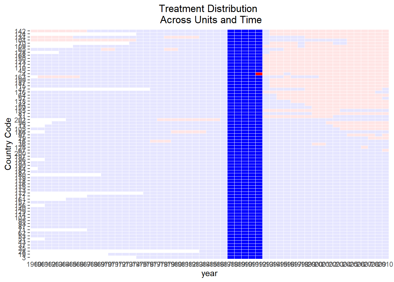
Figure 35.16: Treatment by country and year.

Control units and the treated unit have identical treatment histories over the lag window (1988-1991) (Figure 35.16)

DisplayTreatment(
    legend.position = "none",
    xlab = "year",
    ylab = "Country Code",
    panel.data = PanelData(panel.data = dem, 
              unit.id = "wbcode2", 
              time.id = "year", 
              treatment = "dem", 
              outcome = "y"),
    matched.set = PM.results.none$att[2],
    # highlight the particular set
    show.set.only = TRUE
)

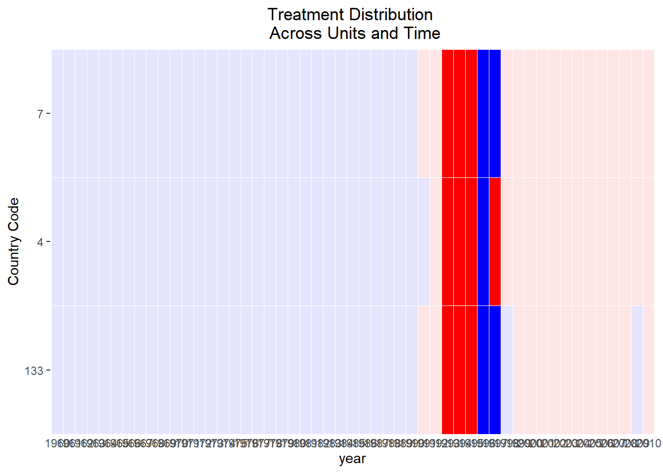
Figure 35.17: Focused treatment visualization.

This set is more limited than the first one, but we can still see that we have exact past histories (Figure 35.17).

• Refining Matched Sets

  • Refinement involves assigning weights to control units.

  • Users must:

    1. Specify a method for calculating unit similarity/distance.

    2. Choose variables for similarity/distance calculations.

• Select a Refinement Method

  • Users determine the refinement method via the refinement.method argument.

  • Options include:

    • mahalanobis
    • ps.match
    • CBPS.match
    • ps.weight
    • CBPS.weight
    • ps.msm.weight
    • CBPS.msm.weight
    • none

  • Methods with “match” in the name and Mahalanobis will assign equal weights to similar control units.

  • “Weighting” methods give higher weights to control units more similar to treated units.

• Variable Selection

  • Users need to define which covariates will be used through the covs.formula argument, a one-sided formula object.

  • Variables on the right side of the formula are used for calculations.

  • “Lagged” versions of variables can be included using the format: I(lag(name.of.var, 0:n)).

• Understanding PanelMatch and matched.set objects

  • The PanelMatch function returns a PanelMatch object.

  • The most crucial element within the PanelMatch object is the matched.set object.

  • Within the PanelMatch object, the matched.set object will have names like att, art, or atc.

  • If qoi = ate, there will be two matched.set objects: att and atc.

• Matched.set Object Details

  • matched.set is a named list with added attributes.

  • Attributes include:

    • Lag

    • Names of treatment

    • Unit and time variables

  • Each list entry represents a matched set of treated and control units.

  • Naming follows a structure: [id variable].[time variable].

  • Each list element is a vector of control unit ids that match the treated unit mentioned in the element name.

  • Since it’s a matching method, weights are only given to the size.match most similar control units based on distance calculations.

# PanelMatch without any refinement
PM.results.none <-
    PanelMatch(
        lag = 4,
        refinement.method = "none",
        panel.data = PanelData(panel.data = dem, 
              unit.id = "wbcode2", 
              time.id = "year", 
              treatment = "dem", 
              outcome = "y"),
        match.missing = TRUE,
        size.match = 5,
        qoi = "att",
        lead = 0:4,
        forbid.treatment.reversal = FALSE,
        use.diagonal.variance.matrix = TRUE
    )

# Extract the matched.set object
msets.none <- PM.results.none$att

# PanelMatch with refinement
PM.results.maha <-
    PanelMatch(
        lag = 4,
        refinement.method = "mahalanobis", # use Mahalanobis distance
        panel.data = PanelData(panel.data = dem, 
              unit.id = "wbcode2", 
              time.id = "year", 
              treatment = "dem", 
              outcome = "y"),
        match.missing = TRUE,
        covs.formula = ~ tradewb,
        size.match = 5,
        qoi = "att" ,
        lead = 0:4,
        forbid.treatment.reversal = FALSE,
        use.diagonal.variance.matrix = TRUE
    )
msets.maha <- PM.results.maha$att

# these 2 should be identical because weights are not shown
msets.none |> head()
#>   wbcode2 year matched.set.size
#> 1       4 1992               74
#> 2       4 1997                2
#> 3       6 1973               63
#> 4       6 1983               73
#> 5       7 1991               81
#> ... [1 more matched set(s) not printed]
msets.maha |> head()
#>   wbcode2 year matched.set.size
#> 1       4 1992               74
#> 2       4 1997                2
#> 3       6 1973               63
#> 4       6 1983               73
#> 5       7 1991               81
#> ... [1 more matched set(s) not printed]
# summary(msets.none)
# summary(msets.maha)

Visualizing Matched Sets with the plot method

• Users can visualize the distribution of the matched set sizes (Figure 35.18).

• A red line, by default, indicates the count of matched sets where treated units had no matching control units (i.e., empty matched sets).

• Plot adjustments can be made using graphics::plot.

plot(
  msets.none,
  panel.data = PanelData(
    panel.data = dem,
    unit.id = "wbcode2",
    time.id = "year",
    treatment = "dem",
    outcome = "y"
  )
)

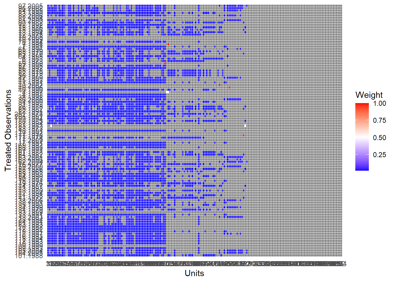
Figure 35.18: Weight distribution across donor units used to construct synthetic control matches.

Comparing Methods of Refinement

• Users are encouraged to:

  • Use substantive knowledge for experimentation and evaluation.

  • Consider the following when configuring PanelMatch:

    1. The number of matched sets.

    2. The number of controls matched to each treated unit.

    3. Achieving covariate balance.

  • Note: Large numbers of small matched sets can lead to larger standard errors during the estimation stage.

  • Covariates that aren’t well balanced can lead to undesirable comparisons between treated and control units.

  • Aspects to consider include:

    • Refinement method.

    • Variables for weight calculation.

    • Size of the lag window.

    • Procedures for addressing missing data (refer to match.missing and listwise.delete arguments).

    • Maximum size of matched sets (for matching methods).

• Supportive Features:

  • print, plot, and summary methods assist in understanding matched sets and their sizes.

  • get_covariate_balance helps evaluate covariate balance:

    • Lower values in the covariate balance calculations are preferred.

PM.results.none <-
    PanelMatch(
        lag = 4,
        refinement.method = "none",
        panel.data = PanelData(panel.data = dem, 
              unit.id = "wbcode2", 
              time.id = "year", 
              treatment = "dem", 
              outcome = "y"),
        match.missing = TRUE,
        size.match = 5,
        qoi = "att",
        lead = 0:4,
        forbid.treatment.reversal = FALSE,
        use.diagonal.variance.matrix = TRUE
    )
PM.results.maha <-
    PanelMatch(
        lag = 4,
        refinement.method = "mahalanobis",
        panel.data = PanelData(panel.data = dem, 
              unit.id = "wbcode2", 
              time.id = "year", 
              treatment = "dem", 
              outcome = "y"),
        match.missing = TRUE,
        covs.formula = ~ I(lag(tradewb, 1:4)) + I(lag(y, 1:4)),
        size.match = 5,
        qoi = "att",
        lead = 0:4,
        forbid.treatment.reversal = FALSE,
        use.diagonal.variance.matrix = TRUE
    )

# listwise deletion used for missing data
PM.results.listwise <-
    PanelMatch(
        lag = 4,
        refinement.method = "mahalanobis",
        panel.data = PanelData(panel.data = dem, 
              unit.id = "wbcode2", 
              time.id = "year", 
              treatment = "dem", 
              outcome = "y"),
        match.missing = FALSE,
        listwise.delete = TRUE,
        covs.formula = ~ I(lag(tradewb, 1:4)) + I(lag(y, 1:4)),
        size.match = 5,
        qoi = "att",
        lead = 0:4,
        forbid.treatment.reversal = FALSE,
        use.diagonal.variance.matrix = TRUE
    )

# propensity score based weighting method
PM.results.ps.weight <-
    PanelMatch(
        lag = 4,
        refinement.method = "ps.weight",
        panel.data = PanelData(panel.data = dem, 
              unit.id = "wbcode2", 
              time.id = "year", 
              treatment = "dem", 
              outcome = "y"),
        match.missing = FALSE,
        listwise.delete = TRUE,
        covs.formula = ~ I(lag(tradewb, 1:4)) + I(lag(y, 1:4)),
        size.match = 5,
        qoi = "att",
        lead = 0:4,
        forbid.treatment.reversal = FALSE
    )

get_covariate_balance(
    PM.results.none,
    panel.data = PanelData(panel.data = dem, 
              unit.id = "wbcode2", 
              time.id = "year", 
              treatment = "dem", 
              outcome = "y"),
    covariates = c("tradewb", "y")
)
#> 
#> ==============================
#> PM.results.none 
#> ==============================
#> 
#> --- QOI: att ---
#>         tradewb            y
#> t_4 -0.07245466  0.291871990
#> t_3 -0.20930129  0.208654876
#> t_2 -0.24425207  0.107736647
#> t_1 -0.10806125 -0.004950238
#> t_0 -0.09493854 -0.015198483

# Compare covariate balance to refined sets
# See large improvement in balance
get_covariate_balance(
    PM.results.ps.weight,
     panel.data = PanelData(panel.data = dem, 
              unit.id = "wbcode2", 
              time.id = "year", 
              treatment = "dem", 
              outcome = "y"),
    covariates = c("tradewb", "y")
)
#> 
#> ==============================
#> PM.results.ps.weight 
#> ==============================
#> 
#> --- QOI: att ---
#>         tradewb          y
#> t_4 0.014362590 0.04035905
#> t_3 0.005529734 0.04188731
#> t_2 0.009410044 0.04195008
#> t_1 0.027907540 0.03975173
#> t_0 0.040272235 0.04167921

PanelEstimate

• Standard Error Calculation Methods

  • There are different methods available:

    • Bootstrap (default method with 1000 iterations).

    • Conditional: Assumes independence across units, but not time.

    • Unconditional: Doesn’t make assumptions of independence across units or time.

  • For qoi values set to att, art, or atc (Imai, Kim, et al. 2021):

    • You can use analytical methods for calculating standard errors, which include both “conditional” and “unconditional” methods.

PE.results <- PanelEstimate(
    sets              = PM.results.ps.weight,
    panel.data = PanelData(panel.data = dem, 
              unit.id = "wbcode2", 
              time.id = "year", 
              treatment = "dem", 
              outcome = "y"),
    se.method         = "bootstrap",
    number.iterations = 1000,
    confidence.level  = .95
)

# point estimates
PE.results[["estimates"]]
#> NULL

# standard errors
PE.results[["standard.error"]]
#>       t+0       t+1       t+2       t+3       t+4 
#> 0.6378008 1.0580194 1.4415817 1.8023301 2.2215475


# use conditional method
PE.results <- PanelEstimate(
    sets             = PM.results.ps.weight,
    panel.data = PanelData(panel.data = dem, 
              unit.id = "wbcode2", 
              time.id = "year", 
              treatment = "dem", 
              outcome = "y"),
    se.method        = "conditional",
    confidence.level = .95
)

# point estimates
PE.results[["estimates"]]
#> NULL

# standard errors
PE.results[["standard.error"]]
#>       t+0       t+1       t+2       t+3       t+4 
#> 0.4844805 0.8170604 1.1171942 1.4116879 1.7172143

summary(PE.results)
#>      estimate std.error       2.5%    97.5%
#> t+0 0.2609565 0.4844805 -0.6886078 1.210521
#> t+1 0.9630847 0.8170604 -0.6383243 2.564494
#> t+2 1.2851017 1.1171942 -0.9045586 3.474762
#> t+3 1.7370930 1.4116879 -1.0297644 4.503950
#> t+4 1.4871846 1.7172143 -1.8784937 4.852863

Figure 35.19 shows the estimated treatment effects over time.

plot(PE.results)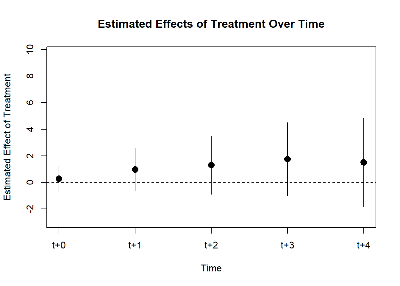

Figure 35.19: Post-treatment effects over time.

Moderating Variables

# moderating variable
dem$moderator <- 0
dem$moderator <- ifelse(dem$wbcode2 > 100, 1, 2)

PM.results <-
    PanelMatch(
        lag                          = 4,
        # time.id                      = "year",
        # unit.id                      = "wbcode2",
        # treatment                    = "dem",
        refinement.method            = "mahalanobis",
        panel.data = PanelData(panel.data = dem, 
              unit.id = "wbcode2", 
              time.id = "year", 
              treatment = "dem", 
              outcome = "y"),
        match.missing                = TRUE,
        covs.formula                 = ~ I(lag(tradewb, 1:4)) + I(lag(y, 1:4)),
        size.match                   = 5,
        qoi                          = "att",
        # outcome.var                  = "y",
        lead                         = 0:4,
        forbid.treatment.reversal    = FALSE,
        use.diagonal.variance.matrix = TRUE
    )
PE.results <-
    PanelEstimate(
        sets      = PM.results,
        panel.data = PanelData(
            panel.data = dem,
            unit.id = "wbcode2",
            time.id = "year",
            treatment = "dem",
            outcome = "y"
        ),
        moderator = "moderator"
    )

Figure 35.20 shows the estimated treatment effects over time by a moderating variable.

# Each element in the list corresponds to a level in the moderator
plot(PE.results[[1]])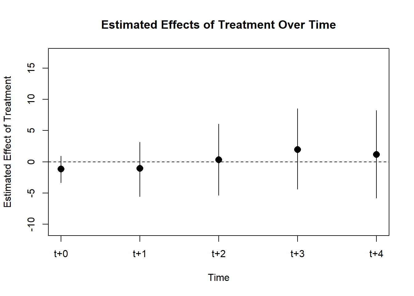

Figure 35.20: Estimated effects of treatment over time.

# plot(PE.results[[2]])

In this study, aligned with the research by Acemoglu et al. (2019), two key effects of democracy on economic growth are estimated: the impact of democratization and that of authoritarian reversal. The treatment variable, \(X_{it}\), is defined to be one if country \(i\) is democratic in year \(t\), and zero otherwise.

The Average Treatment Effect for the Treated (ATT) under democratization is formulated as follows:

\[ \begin{aligned} \delta(F, L) &= \mathbb{E} \left\{ Y_{i, t + F} (X_{it} = 1, X_{i, t - 1} = 0, \{X_{i,t-l}\}_{l=2}^L) \right. \\ &\left. - Y_{i, t + F} (X_{it} = 0, X_{i, t - 1} = 0, \{X_{i,t-l}\}_{l=2}^L) | X_{it} = 1, X_{i, t - 1} = 0 \right\} \end{aligned} \]

In this framework, the treated observations are countries that transition from an authoritarian regime \(X_{it-1} = 0\) to a democratic one \(X_{it} = 1\). The variable \(F\) represents the number of leads, denoting the time periods following the treatment, and \(L\) signifies the number of lags, indicating the time periods preceding the treatment.

The ATT under authoritarian reversal is given by:

\[ \begin{aligned} &\mathbb{E} \left[ Y_{i, t + F} (X_{it} = 0, X_{i, t - 1} = 1, \{ X_{i, t - l}\}_{l=2}^L ) \right. \\ &\left. - Y_{i, t + F} (X_{it} = 1, X_{it-1} = 1, \{X_{i, t - l} \}_{l=2}^L ) | X_{it} = 0, X_{i, t - 1} = 1 \right] \end{aligned} \]

The ATT is calculated conditioning on 4 years of lags (\(L = 4\)) and up to 4 years following the policy change \(F = 1, 2, 3, 4\). Matched sets for each treated observation are constructed based on its treatment history, with the number of matched control units generally decreasing when considering a 4-year treatment history as compared to a 1-year history.

To enhance the quality of matched sets, methods such as Mahalanobis distance matching, propensity score matching, and propensity score weighting are utilized. These approaches enable us to evaluate the effectiveness of each refinement method. In the process of matching, we employ both up-to-five and up-to-ten matching to investigate how sensitive our empirical results are to the maximum number of allowed matches. For more information on the refinement process, please see the Web Appendix.

The Mahalanobis distance is expressed through a specific formula. We aim to pair each treated unit with a maximum of \(J\) control units, permitting replacement, denoted as \(| \mathcal{M}_{it} \le J|\). The average Mahalanobis distance between a treated and each control unit over time is computed as:

\[ S_{it} (i') = \frac{1}{L} \sum_{l = 1}^L \sqrt{(\mathbf{V}_{i, t - l} - \mathbf{V}_{i', t -l})^T \mathbf{\Sigma}_{i, t - l}^{-1} (\mathbf{V}_{i, t - l} - \mathbf{V}_{i', t -l})} \]

For a matched control unit \(i' \in \mathcal{M}_{it}\), \(\mathbf{V}_{it'}\) represents the time-varying covariates to adjust for, and \(\mathbf{\Sigma}_{it'}\) is the sample covariance matrix for \(\mathbf{V}_{it'}\). Essentially, we calculate a standardized distance using time-varying covariates and average this across different time intervals.

In the context of propensity score matching, we employ a logistic regression model with balanced covariates to derive the propensity score. Defined as the conditional likelihood of treatment given pre-treatment covariates (Rosenbaum and Rubin 1983), the propensity score is estimated by first creating a data subset comprised of all treated and their matched control units from the same year. This logistic regression model is then fitted as follows:

\[ \begin{aligned} & e_{it} (\{\mathbf{U}_{i, t - l} \}^L_{l = 1}) \\ &= Pr(X_{it} = 1| \mathbf{U}_{i, t -1}, \ldots, \mathbf{U}_{i, t - L}) \\ &= \frac{1}{1 = \exp(- \sum_{l = 1}^L \beta_l^T \mathbf{U}_{i, t - l})} \end{aligned} \]

where \(\mathbf{U}_{it'} = (X_{it'}, \mathbf{V}_{it'}^T)^T\). Given this model, the estimated propensity score for all treated and matched control units is then computed. This enables the adjustment for lagged covariates via matching on the calculated propensity score, resulting in the following distance measure:

\[ S_{it} (i') = | \text{logit} \{ \hat{e}_{it} (\{ \mathbf{U}_{i, t - l}\}^L_{l = 1})\} - \text{logit} \{ \hat{e}_{i't}( \{ \mathbf{U}_{i', t - l} \}^L_{l = 1})\} | \]

Here, \(\hat{e}_{i't} (\{ \mathbf{U}_{i, t - l}\}^L_{l = 1})\) represents the estimated propensity score for each matched control unit \(i' \in \mathcal{M}_{it}\).

Once the distance measure \(S_{it} (i')\) has been determined for all control units in the original matched set, we fine-tune this set by selecting up to \(J\) closest control units, which meet a researcher-defined caliper constraint \(C\). All other control units receive zero weight. This results in a refined matched set for each treated unit \((i, t)\):

\[ \mathcal{M}_{it}^* = \{i' : i' \in \mathcal{M}_{it}, S_{it} (i') < C, S_{it} \le S_{it}^{(J)}\} \]

\(S_{it}^{(J)}\) is the \(J\)th smallest distance among the control units in the original set \(\mathcal{M}_{it}\).

For further refinement using weighting, a weight is assigned to each control unit \(i'\) in a matched set corresponding to a treated unit \((i, t)\), with greater weight accorded to more similar units. We utilize inverse propensity score weighting, based on the propensity score model mentioned earlier:

\[ w_{it}^{i'} \propto \frac{\hat{e}_{i't} (\{ \mathbf{U}_{i, t-l} \}^L_{l = 1} )}{1 - \hat{e}_{i't} (\{ \mathbf{U}_{i, t-l} \}^L_{l = 1} )} \]

In this model, \(\sum_{i' \in \mathcal{M}_{it}} w_{it}^{i'} = 1\) and \(w_{it}^{i'} = 0\) for \(i' \notin \mathcal{M}_{it}\). The model is fitted to the complete sample of treated and matched control units.

Checking Covariate Balance A distinct advantage of the proposed methodology over regression methods is the ability it offers researchers to inspect the covariate balance between treated and matched control observations. This facilitates the evaluation of whether treated and matched control observations are comparable regarding observed confounders. To investigate the mean difference of each covariate (e.g., \(V_{it'j}\), representing the \(j\)-th variable in \(\mathbf{V}_{it'}\)) between the treated observation and its matched control observation at each pre-treatment time period (i.e., \(t' < t\)), we further standardize this difference. For any given pretreatment time period, we adjust by the standard deviation of each covariate across all treated observations in the dataset. Thus, the mean difference is quantified in terms of standard deviation units. Formally, for each treated observation \((i,t)\) where \(D_{it} = 1\), we define the covariate balance for variable \(j\) at the pretreatment time period \(t - l\) as: \[\begin{equation} B_{it}(j, l) = \frac{V_{i, t- l,j}- \sum_{i' \in \mathcal{M}_{it}}w_{it}^{i'}V_{i', t-l,j}}{\sqrt{\frac{1}{N_1 - 1} \sum_{i'=1}^N \sum_{t' = L+1}^{T-F}D_{i't'}(V_{i', t'-l, j} - \bar{V}_{t' - l, j})^2}} \label{eq:covbalance} \end{equation}\] where \(N_1 = \sum_{i'= 1}^N \sum_{t' = L+1}^{T-F} D_{i't'}\) denotes the total number of treated observations and \(\bar{V}_{t-l,j} = \sum_{i=1}^N D_{i,t-l,j}/N\). We then aggregate this covariate balance measure across all treated observations for each covariate and pre-treatment time period:

\[\begin{equation} \bar{B}(j, l) = \frac{1}{N_1} \sum_{i=1}^N \sum_{t = L+ 1}^{T-F}D_{it} B_{it}(j,l) \label{eq:aggbalance} \end{equation}\]

Lastly, we evaluate the balance of lagged outcome variables over several pre-treatment periods and that of time-varying covariates. This examination aids in assessing the validity of the parallel trend assumption integral to the DiD estimator justification.

In the balance scatter figure, we demonstrate the enhancement of covariate balance thanks to the refinement of matched sets. Each scatter plot contrasts the absolute standardized mean difference between before (horizontal axis) and after (vertical axis) this refinement. Points below the 45-degree line indicate an improved standardized mean balance for certain time-varying covariates post-refinement. The majority of variables benefit from this refinement process. Notably, the propensity score weighting (bottom panel) shows the most significant improvement, whereas Mahalanobis matching (top panel) yields a more modest improvement.

library(PanelMatch)
library(causalverse)

runPanelMatch <- function(method, lag, size.match=NULL, qoi="att") {
    
    # Default parameters for PanelMatch
    common.args <- list(
        lag = lag,
        panel.data = PanelData(panel.data = dem, 
              unit.id = "wbcode2", 
              time.id = "year", 
              treatment = "dem", 
              outcome = "y"),
        covs.formula = ~ I(lag(tradewb, 1:4)) + I(lag(y, 1:4)),
        qoi = qoi,
        lead = 0:4,
        forbid.treatment.reversal = FALSE,
        size.match = size.match  # setting size.match here for all methods
    )
    
    if(method == "mahalanobis") {
        common.args$refinement.method <- "mahalanobis"
        common.args$match.missing <- TRUE
        common.args$use.diagonal.variance.matrix <- TRUE
    } else if(method == "ps.match") {
        common.args$refinement.method <- "ps.match"
        common.args$match.missing <- FALSE
        common.args$listwise.delete <- TRUE
    } else if(method == "ps.weight") {
        common.args$refinement.method <- "ps.weight"
        common.args$match.missing <- FALSE
        common.args$listwise.delete <- TRUE
    }
    
    return(do.call(PanelMatch, common.args))
}

methods <- c("mahalanobis", "ps.match", "ps.weight")
lags <- c(1, 4)
sizes <- c(5, 10)

You can either do it sequentially

res_pm <- list()

for(method in methods) {
    for(lag in lags) {
        for(size in sizes) {
            name <- paste0(method, ".", lag, "lag.", size, "m")
            res_pm[[name]] <- runPanelMatch(method, lag, size)
        }
    }
}

# Now, you can access res_pm using res_pm[["mahalanobis.1lag.5m"]] etc.

# for treatment reversal
res_pm_rev <- list()

for(method in methods) {
    for(lag in lags) {
        for(size in sizes) {
            name <- paste0(method, ".", lag, "lag.", size, "m")
            res_pm_rev[[name]] <- runPanelMatch(method, lag, size, qoi = "art")
        }
    }
}

or in parallel

library(foreach)
library(doParallel)
registerDoParallel(cores = 4)
# Initialize an empty list to store results
res_pm <- list()

# Replace nested for-loops with foreach
results <-
  foreach(
    method = methods,
    .combine = 'c',
    .multicombine = TRUE,
    .packages = c("PanelMatch", "causalverse")
  ) %dopar% {
    tmp <- list()
    for (lag in lags) {
      for (size in sizes) {
        name <- paste0(method, ".", lag, "lag.", size, "m")
        tmp[[name]] <- runPanelMatch(method, lag, size)
      }
    }
    tmp
  }

# Collate results
for (name in names(results)) {
  res_pm[[name]] <- results[[name]]
}

# Treatment reversal
# Initialize an empty list to store results
res_pm_rev <- list()

# Replace nested for-loops with foreach
results_rev <-
  foreach(
    method = methods,
    .combine = 'c',
    .multicombine = TRUE,
    .packages = c("PanelMatch", "causalverse")
  ) %dopar% {
    tmp <- list()
    for (lag in lags) {
      for (size in sizes) {
        name <- paste0(method, ".", lag, "lag.", size, "m")
        tmp[[name]] <-
          runPanelMatch(method, lag, size, qoi = "art")
      }
    }
    tmp
  }

# Collate results
for (name in names(results_rev)) {
  res_pm_rev[[name]] <- results_rev[[name]]
}


stopImplicitCluster()

The export script below assembles the per-method balance scatter plots (Mahalanobis, PS matching, PS weighting at 1- and 4-year lags) into a single PNG that is rendered above.

library(gridExtra)

# Updated plotting function
create_balance_plot <- function(method, lag, sizes, res_pm, dem) {
    matched_set_lists <- lapply(sizes, function(size) {
        res_pm[[paste0(method, ".", lag, "lag.", size, "m")]]$att
    })
    
    return(
        balance_scatter_custom(
            matched_set_list = matched_set_lists,
            legend.title = "Possible Matches",
            set.names = as.character(sizes),
            legend.position = c(0.2, 0.8),
            
            # for compiled plot, you don't need x,y, or main labs
            x.axis.label = "",
            y.axis.label = "",
            main = "",
            data = dem,
            dot.size = 5,
            # show.legend = F,
            them_use = causalverse::ama_theme(base_size = 32),
            covariates = c("y", "tradewb")
        )
    )
}

plots <- list()

for (method in methods) {
    for (lag in lags) {
        plots[[paste0(method, ".", lag, "lag")]] <-
            create_balance_plot(method, lag, sizes, res_pm, dem)
    }
}

# # Arranging plots in a 3x2 grid
# grid.arrange(plots[["mahalanobis.1lag"]],
#              plots[["mahalanobis.4lag"]],
#              plots[["ps.match.1lag"]],
#              plots[["ps.match.4lag"]],
#              plots[["ps.weight.1lag"]],
#              plots[["ps.weight.4lag"]],
#              ncol=2, nrow=3)


# Standardized Mean Difference of Covariates
library(gridExtra)
library(grid)

# Create column and row labels using textGrob
col_labels <- c("1-year Lag", "4-year Lag")
row_labels <- c("Maha Matching", "PS Matching", "PS Weigthing")

major.axes.fontsize = 40
minor.axes.fontsize = 30

png(
    file.path(getwd(), "images", "did_balance_scatter.png"),
    width = 1200,
    height = 1000
)

# Create a list-of-lists, where each inner list represents a row
grid_list <- list(
    list(
        nullGrob(),
        textGrob(col_labels[1], gp = gpar(fontsize = minor.axes.fontsize)),
        textGrob(col_labels[2], gp = gpar(fontsize = minor.axes.fontsize))
    ),
    
    list(textGrob(
        row_labels[1],
        gp = gpar(fontsize = minor.axes.fontsize),
        rot = 90
    ), plots[["mahalanobis.1lag"]], plots[["mahalanobis.4lag"]]),
    
    list(textGrob(
        row_labels[2],
        gp = gpar(fontsize = minor.axes.fontsize),
        rot = 90
    ), plots[["ps.match.1lag"]], plots[["ps.match.4lag"]]),
    
    list(textGrob(
        row_labels[3],
        gp = gpar(fontsize = minor.axes.fontsize),
        rot = 90
    ), plots[["ps.weight.1lag"]], plots[["ps.weight.4lag"]])
)

# "Flatten" the list-of-lists into a single list of grobs
grobs <- do.call(c, grid_list)

grid.arrange(
    grobs = grobs,
    ncol = 3,
    nrow = 4,
    widths = c(0.15, 0.42, 0.42),
    heights = c(0.15, 0.28, 0.28, 0.28)
)

grid.text(
    "Before Refinement",
    x = 0.5,
    y = 0.03,
    gp = gpar(fontsize = major.axes.fontsize)
)
grid.text(
    "After Refinement",
    x = 0.03,
    y = 0.5,
    rot = 90,
    gp = gpar(fontsize = major.axes.fontsize)
)
dev.off()

Figure 35.21 compares covariate balance across refinement methods and lag lengths.

knitr::include_graphics(file.path(getwd(), "images", "did_balance_scatter.png"))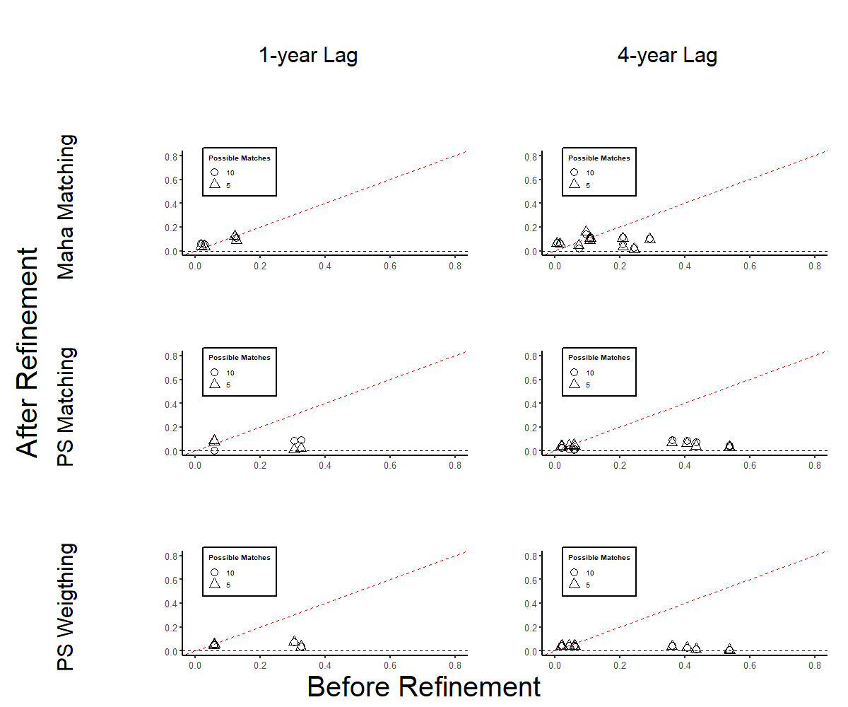

Figure 35.21: Variable balance after matched-set refinement.

Note: Scatter plots display the standardized mean difference of each covariate \(j\) and lag year \(l\) before (x-axis) and after (y-axis) matched set refinement. Each plot includes varying numbers of possible matches for each matching method. Rows represent different matching/weighting methods, while columns indicate adjustments for various lag lengths. Figure 35.22 below repeats the exercise for the pre-treatment period under a richer set of refinement configurations.

# Step 1: Define configurations
configurations <- list(
    list(refinement.method = "none", qoi = "att"),
    list(refinement.method = "none", qoi = "art"),
    list(refinement.method = "mahalanobis", qoi = "att"),
    list(refinement.method = "mahalanobis", qoi = "art"),
    list(refinement.method = "ps.match", qoi = "att"),
    list(refinement.method = "ps.match", qoi = "art"),
    list(refinement.method = "ps.weight", qoi = "att"),
    list(refinement.method = "ps.weight", qoi = "art")
)

# Step 2: Use lapply or loop to generate results
results <- lapply(configurations, function(config) {
    PanelMatch(
        lag                       = 4,
        panel.data = PanelData(panel.data = dem, 
              unit.id = "wbcode2", 
              time.id = "year", 
              treatment = "dem", 
              outcome = "y"),
        match.missing             = FALSE,
        listwise.delete           = TRUE,
        size.match                = 5,
        lead                      = 0:4,
        forbid.treatment.reversal = FALSE,
        refinement.method         = config$refinement.method,
        covs.formula              = ~ I(lag(tradewb, 1:4)) + I(lag(y, 1:4)),
        qoi                       = config$qoi
    )
})

# Step 3: Get covariate balance and plot
plots <- mapply(function(result, config) {
    df <- get_covariate_balance(
        if (config$qoi == "att")
            result$att
        else
            result$art,
        panel.data = PanelData(panel.data = dem, 
              unit.id = "wbcode2", 
              time.id = "year", 
              treatment = "dem", 
              outcome = "y"),
        covariates = c("tradewb", "y"),
        plot = F
    )
    causalverse::plot_covariate_balance_pretrend(df, main = "", show_legend = F)
}, results, configurations, SIMPLIFY = FALSE)

# Set names for plots
names(plots) <- sapply(configurations, function(config) {
    paste(config$qoi, config$refinement.method, sep = ".")
})

The script below assembles the per-method, per-estimand pre-treatment balance plots into a single composite PNG used by the rendered figure above.

library(gridExtra)
library(grid)

# Column and row labels
col_labels <-
    c("None",
      "Mahalanobis",
      "Propensity Score Matching",
      "Propensity Score Weighting")
row_labels <- c("ATT", "ART")

# Specify your desired fontsize for labels
minor.axes.fontsize <- 16
major.axes.fontsize <- 20

png(file.path(getwd(), "images", "p_covariate_balance.png"), width=1200, height=1000)

# Create a list-of-lists, where each inner list represents a row
grid_list <- list(
    list(
        nullGrob(),
        textGrob(col_labels[1], gp = gpar(fontsize = minor.axes.fontsize)),
        textGrob(col_labels[2], gp = gpar(fontsize = minor.axes.fontsize)),
        textGrob(col_labels[3], gp = gpar(fontsize = minor.axes.fontsize)),
        textGrob(col_labels[4], gp = gpar(fontsize = minor.axes.fontsize))
    ),
    
    list(
        textGrob(
            row_labels[1],
            gp = gpar(fontsize = minor.axes.fontsize),
            rot = 90
        ),
        plots$att.none,
        plots$att.mahalanobis,
        plots$att.ps.match,
        plots$att.ps.weight
    ),
    
    list(
        textGrob(
            row_labels[2],
            gp = gpar(fontsize = minor.axes.fontsize),
            rot = 90
        ),
        plots$art.none,
        plots$art.mahalanobis,
        plots$art.ps.match,
        plots$art.ps.weight
    )
)

# "Flatten" the list-of-lists into a single list of grobs
grobs <- do.call(c, grid_list)

# Arrange your plots with text labels
grid.arrange(
    grobs   = grobs,
    ncol    = 5,
    nrow    = 3,
    widths  = c(0.1, 0.225, 0.225, 0.225, 0.225),
    heights = c(0.1, 0.45, 0.45)
)

# Add main x and y axis titles
grid.text(
    "Refinement Methods",
    x  = 0.5,
    y  = 0.01,
    gp = gpar(fontsize = major.axes.fontsize)
)
grid.text(
    "Quantities of Interest",
    x   = 0.02,
    y   = 0.5,
    rot = 90,
    gp  = gpar(fontsize = major.axes.fontsize)
)

dev.off()

knitr::include_graphics(file.path(getwd(), "images", "p_covariate_balance.png"))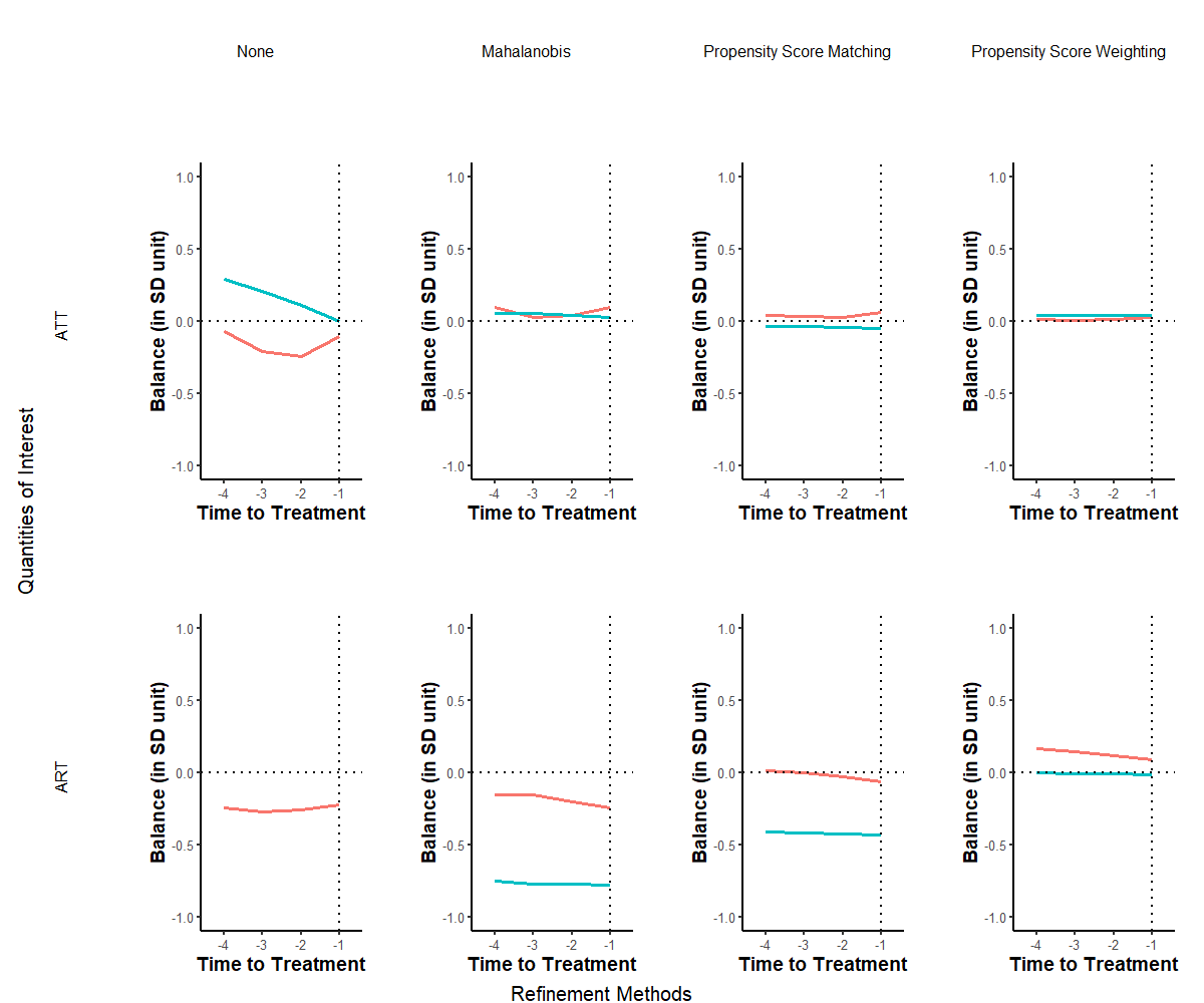

Figure 35.22: Covariate balance over time by refinement method and estimand.

Note: Each graph displays the standardized mean difference plotted on the vertical axis across a pre-treatment duration of four years represented on the horizontal axis. The leftmost column illustrates the balance prior to refinement, while the subsequent three columns depict the covariate balance post the application of distinct refinement techniques. Each individual line signifies the balance of a specific variable during the pre-treatment phase. The red line is tradewb and blue line is the lagged outcome variable.

In Figure 35.22, we observe a marked improvement in covariate balance due to the implemented matching procedures during the pre-treatment period. Our analysis prioritizes methods that adjust for time-varying covariates over a span of four years preceding the treatment initiation. The two rows delineate the standardized mean balance for both treatment modalities, with individual lines representing the balance for each covariate.

Across all scenarios, the refinement attributed to matched sets significantly enhances balance. Notably, using propensity score weighting considerably mitigates imbalances in confounders. While some degree of imbalance remains evident in the Mahalanobis distance and propensity score matching techniques, the standardized mean difference for the lagged outcome remains stable throughout the pre-treatment phase. This consistency lends credence to the validity of the proposed DiD estimator.

Estimation Results

We now detail the estimated ATTs derived from the matching techniques. Figure below offers visual representations of the impacts of treatment initiation (upper panel) and treatment reversal (lower panel) on the outcome variable for a duration of 5 years post-transition, specifically, (\(F = 0, 1, …, 4\)). Across the five methods (columns), it becomes evident that the point estimates of effects associated with treatment initiation consistently approximate zero over the 5-year window. In contrast, the estimated outcomes of treatment reversal are notably negative and maintain statistical significance through all refinement techniques during the initial year of transition and the 1 to 4 years that follow, provided treatment reversal is permissible. These effects are notably pronounced, pointing to an estimated reduction of roughly X% in the outcome variable.

Collectively, these findings indicate that the transition into the treated state from its absence doesn’t invariably lead to a heightened outcome. Instead, the transition from the treated state back to its absence exerts a considerable negative effect on the outcome variable in both the short and intermediate terms. Hence, the positive effect of the treatment (if we were to use traditional DiD) is actually driven by the negative effect of treatment reversal.

# sequential
# Step 1: Apply PanelEstimate function

# Initialize an empty list to store results
res_est <- vector("list", length(res_pm))

# Iterate over each element in res_pm
for (i in 1:length(res_pm)) {
  res_est[[i]] <- PanelEstimate(
    res_pm[[i]],
    data = dem,
    se.method = "bootstrap",
    number.iterations = 1000,
    confidence.level = .95
  )
  # Transfer the name of the current element to the res_est list
  names(res_est)[i] <- names(res_pm)[i]
}

# Step 2: Apply plot_PanelEstimate function

# Initialize an empty list to store plot results
res_est_plot <- vector("list", length(res_est))

# Iterate over each element in res_est
for (i in 1:length(res_est)) {
    res_est_plot[[i]] <-
        plot_PanelEstimate(res_est[[i]],
                           main = "",
                           theme_use = causalverse::ama_theme(base_size = 14))
    # Transfer the name of the current element to the res_est_plot list
    names(res_est_plot)[i] <- names(res_est)[i]
}

# check results
# res_est_plot$mahalanobis.1lag.5m


# Step 1: Apply PanelEstimate function for res_pm_rev

# Initialize an empty list to store results
res_est_rev <- vector("list", length(res_pm_rev))

# Iterate over each element in res_pm_rev
for (i in 1:length(res_pm_rev)) {
  res_est_rev[[i]] <- PanelEstimate(
    res_pm_rev[[i]],
    data = dem,
    se.method = "bootstrap",
    number.iterations = 1000,
    confidence.level = .95
  )
  # Transfer the name of the current element to the res_est_rev list
  names(res_est_rev)[i] <- names(res_pm_rev)[i]
}

# Step 2: Apply plot_PanelEstimate function for res_est_rev

# Initialize an empty list to store plot results
res_est_plot_rev <- vector("list", length(res_est_rev))

# Iterate over each element in res_est_rev
for (i in 1:length(res_est_rev)) {
    res_est_plot_rev[[i]] <-
        plot_PanelEstimate(res_est_rev[[i]],
                           main = "",
                           theme_use = causalverse::ama_theme(base_size = 14))
  # Transfer the name of the current element to the res_est_plot_rev list
  names(res_est_plot_rev)[i] <- names(res_est_rev)[i]
}

# parallel
library(doParallel)
library(foreach)

# Detect the number of cores to use for parallel processing
num_cores <- 4

# Register the parallel backend
cl <- makeCluster(num_cores)
registerDoParallel(cl)

# Step 1: Apply PanelEstimate function in parallel
res_est <-
    foreach(i = 1:length(res_pm), .packages = "PanelMatch") %dopar% {
        PanelEstimate(
            res_pm[[i]],
            data = dem,
            se.method = "bootstrap",
            number.iterations = 1000,
            confidence.level = .95
        )
    }

# Transfer names from res_pm to res_est
names(res_est) <- names(res_pm)

# Step 2: Apply plot_PanelEstimate function in parallel
res_est_plot <-
    foreach(
        i = 1:length(res_est),
        .packages = c("PanelMatch", "causalverse", "ggplot2")
    ) %dopar% {
        plot_PanelEstimate(res_est[[i]],
                           main = "",
                           theme_use = causalverse::ama_theme(base_size = 10))
    }

# Transfer names from res_est to res_est_plot
names(res_est_plot) <- names(res_est)



# Step 1: Apply PanelEstimate function for res_pm_rev in parallel
res_est_rev <-
    foreach(i = 1:length(res_pm_rev), .packages = "PanelMatch") %dopar% {
        PanelEstimate(
            res_pm_rev[[i]],
            data = dem,
            se.method = "bootstrap",
            number.iterations = 1000,
            confidence.level = .95
        )
    }

# Transfer names from res_pm_rev to res_est_rev
names(res_est_rev) <- names(res_pm_rev)

# Step 2: Apply plot_PanelEstimate function for res_est_rev in parallel
res_est_plot_rev <-
    foreach(
        i = 1:length(res_est_rev),
        .packages = c("PanelMatch", "causalverse", "ggplot2")
    ) %dopar% {
        plot_PanelEstimate(res_est_rev[[i]],
                           main = "",
                           theme_use = causalverse::ama_theme(base_size = 10))
    }

# Transfer names from res_est_rev to res_est_plot_rev
names(res_est_plot_rev) <- names(res_est_rev)

# Stop the cluster
stopCluster(cl)

The export script below assembles the ATT and ART event-study estimates from PanelMatch under five refinement-by-match-size combinations into a composite PNG.

library(gridExtra)
library(grid)

# Column and row labels
col_labels <- c("Mahalanobis 5m",
                "Mahalanobis 10m",
                "PS Matching 5m",
                "PS Matching 10m",
                "PS Weighting 5m")

row_labels <- c("ATT", "ART")

# Specify your desired fontsize for labels
minor.axes.fontsize <- 16
major.axes.fontsize <- 20

png(file.path(getwd(), "images", "p_did_est_in_n_out.png"), width=1200, height=1000)

# Create a list-of-lists, where each inner list represents a row
grid_list <- list(
  list(
    nullGrob(),
    textGrob(col_labels[1], gp = gpar(fontsize = minor.axes.fontsize)),
    textGrob(col_labels[2], gp = gpar(fontsize = minor.axes.fontsize)),
    textGrob(col_labels[3], gp = gpar(fontsize = minor.axes.fontsize)),
    textGrob(col_labels[4], gp = gpar(fontsize = minor.axes.fontsize)),
    textGrob(col_labels[5], gp = gpar(fontsize = minor.axes.fontsize))
  ),
  
  list(
    textGrob(row_labels[1], gp = gpar(fontsize = minor.axes.fontsize), rot = 90),
    res_est_plot$mahalanobis.1lag.5m,
    res_est_plot$mahalanobis.1lag.10m,
    res_est_plot$ps.match.1lag.5m,
    res_est_plot$ps.match.1lag.10m,
    res_est_plot$ps.weight.1lag.5m
  ),
  
  list(
    textGrob(row_labels[2], gp = gpar(fontsize = minor.axes.fontsize), rot = 90),
    res_est_plot_rev$mahalanobis.1lag.5m,
    res_est_plot_rev$mahalanobis.1lag.10m,
    res_est_plot_rev$ps.match.1lag.5m,
    res_est_plot_rev$ps.match.1lag.10m,
    res_est_plot_rev$ps.weight.1lag.5m
  )
)

# "Flatten" the list-of-lists into a single list of grobs
grobs <- do.call(c, grid_list)

# Arrange your plots with text labels
grid.arrange(
  grobs   = grobs,
  ncol    = 6,
  nrow    = 3,
  widths  = c(0.1, 0.18, 0.18, 0.18, 0.18, 0.18),
  heights = c(0.1, 0.45, 0.45)
)

# Add main x and y axis titles
grid.text(
  "Methods",
  x  = 0.5,
  y  = 0.02,
  gp = gpar(fontsize = major.axes.fontsize)
)
grid.text(
  "",
  x   = 0.02,
  y   = 0.5,
  rot = 90,
  gp  = gpar(fontsize = major.axes.fontsize)
)

dev.off()

---

35.12.5 Counterfactual Estimators

Where Panel Match (Section 35.12.4) attacks model dependence by replacing the regression with local matched comparisons, counterfactual estimators take the opposite philosophical route: they keep an explicit outcome model but fit it only on control observations, then use it to impute the missing treated counterfactual. The two strategies are complements rather than substitutes. Counterfactual estimators dominate when the analyst is willing to model \(Y(0)\) but unwilling to extrapolate from treated units; Panel Match dominates when even the \(Y(0)\) model feels suspect and exact treatment-history matches are available.

Counterfactual (or imputation) estimators treat the treated outcome as missing and impute it using information from the control units (Liu et al. 2024). Formally, let

\[Y_{it}(1) \text{ and } Y_{it}(0)\]

denote the potential outcomes for unit \(i\) at time \(t\) with and without treatment. For treated units we only observe \(Y_{it}(1)\), so the goal is to impute the unobserved \(Y_{it}(0)\) (i.e., the counterfactual).

Why use counterfactual estimators?

• Avoid negative weights: unlike some TWFE specifications that generate undesirable extrapolation weights, imputation uses only control data when building the prediction model and (typically) applies equal weights in post-treatment periods.

• Model flexibility: analysts may combine rich time-series structure, non-linear regressions, or machine-learning learners while relaxing the strict exogeneity assumption that plagues TWFE.

• Transparent diagnostics: pre-treatment prediction error (e.g. \(\text{RMSE}_{\text{pre}}\)) offers a concrete check of model fit, something ordinary DiD lacks.

The main families of counterfactual estimators are summarised in Table 35.8.

Table 35.8: Main families of counterfactual (imputation) estimators for DiD: core idea, typical assumptions, and R implementations.

Method	Core idea	Typical assumptions	R implementation
Fixed-effects counterfactual estimator (FEct)	Predict \(Y_{it}(0)\) with two-way additive FEs; compare each treated \(\hat{Y}_{it}(0)\) with \(Y_{it}(1)\)	Linearity; unit and time additive unobservables; no time-varying confounders	fect::fect() or gsynth::gsynth(type = "fe")
Interactive Fixed Effects counterfactual estimator (IFEct) Xu (2017)	Augment FEct with low-rank latent factors: \(Y_{it}(0)=\alpha_i+\gamma_t+\lambda_i^\top f_t+\varepsilon_{it}\)	Low-rank factor structure; factors capture all time-varying confounders	gsynth (default), fixest::feols() with sunab()
Matrix Completion (MC)	Solve a soft-impute nuclear-norm regularization \[\min_{\widehat Y(0)} \|M\odot(Y-\widehat Y(0))\|_F^2 + \lambda\|\widehat Y(0)\|_*\]	Same as IFE but allows dense weak factors; tuning via cross-validation	softImpute, synthdid::mc(), gsynth(type = "mc")
Synthetic Control (SC)	Choose non-negative weights that make the weighted control path mimic a treated path pre-treatment	No interference; convex hull captures counterfactual; no return to pre-treat status	Synth, synthdid, tidysynth, augsynth

---

1. Fixed-Effects Counterfactual Estimator (FEct)

DiD is a special case where each treated observation is compared to the average control outcome. This estimator assumes additive functional form of unobservables based on unit and time FEs. FEct predicts

\[ \widehat{Y}_{it}(0) = \hat{\alpha}_i + \hat{\gamma}_t \]

using only control units when fitting \((\hat{\alpha}_i,\hat{\gamma}_t)\). The ATT is then

\[ \widehat{\tau}_{FEct} = \frac{1}{| \mathcal{T} |}\sum_{(i,t)\in\mathcal T} \{Y_{it}(1)-\widehat{Y}_{it}(0)\}, \]

where \(\mathcal T\) indexes treated unit–time pairs. FEct fixes the improper weighting of TWFE by comparing within each matched pair (where each pair is the treated observation and its predicted counterfactual that is the weighted sum of all untreated observations).

---

2. Interactive Fixed Effects (IFEct)

IFEct generalizes FEct by introducing \(R\) latent factors:

\[ Y_{it}(0) = \alpha_i + \gamma_t + \sum_{r=1}^R \lambda_{ir} f_{tr} + \varepsilon_{it}, \]

estimated via iterative principal components Xu (2017). When we suspect unobserved time-varying confounder, FEct fails. Instead, IFEct uses the factor-augmented models to relax the strict exogeneity assumption where the effects of unobservables can be decomposed to unit FE + time FE + unit x time FE.

Setting \(R=0\) recovers FEct. Generalized Synthetic Control (GSC) (Xu 2017) is an IFEct implementation with ridge penalization when \(R>0\) (This estimator assumes treatments don’t revert).

---

3. Matrix Completion

This is a generalization of factor-augmented models. Rather than fixing \(R\), MC solves a convex optimization where the nuclear-norm penalty \(|\widehat Y(0)|_*\) shrinks all singular values. Different from IFEct which uses hard impute, MC uses soft impute to regularize the singular values when decomposing the residual matrix.

IFEct can outperform MC when the latent factors (of unobservables) are indeed low-rank/sparse and strong; MC prevails when unobservables are dense and weak.

---

4. Synthetic Control

SC is best viewed as a case-study tool (single or few treated units, single treatment onset) unlike FEct/IFEct/MC which handle staggered or many-treated designs naturally.

Take-away: Start with FEct; inspect fit. If time-varying bias remains, graduate to IFEct or MC. Reserve SC for small-\(N\) case studies with clean interventions.

---

Identifying Assumptions:

1. Function Form: Additive separability of observables, unobservables, and idiosyncratic error term.
   • Hence, these models are scale dependent (Athey and Imbens 2006) (e.g., log-transform outcome can invalidate this assumption).
2. Strict Exogeneity: Conditional on observables and unobservables, potential outcomes are independent of treatment assignment (i.e., baseline quasi-randomization)
   • In DiD, where unobservables = unit + time FEs, this assumption is the parallel trends assumption
3. Low-dimensional Decomposition (Feasibility Assumption): Unobservable effects can be decomposed in low-dimension.
   • For the case that \(U_{it} = f_t \times \lambda_i\) where \(f_t\) = common time trend (time FE), and \(\lambda_i\) = unit heterogeneity (unit FE). If \(U_{it} = f_t \times \lambda_i\) , DiD can satisfy this assumption. But this assumption is weaker than that of DID, and allows us to control for unobservables based on data.

Estimation Procedure:

1. Using all control observations, estimate the functions of both observable and unobservable variables (relying on Assumptions 1 and 3).
2. Predict the counterfactual outcomes for each treated unit using the obtained functions.
3. Calculate the difference in treatment effect for each treated individual.
4. By averaging over all treated individuals, you can obtain the Average Treatment Effect on the Treated (ATT).

Notes:

• Use jackknife when number of treated units is small (Liu et al. 2024, 166).

35.12.5.0.1 Imputation Method

Liu et al. (2024) can also account for treatment reversals and heterogeneous treatment effects.

Other imputation estimators include

• Two-stage DiD Estimator (Gardner 2022; Borusyak et al. 2024)

• (Brown et al. 2023)

The code below fits the FECT model and reports pre-treatment F-test diagnostics for the democracy-and-trade panel under a two-way fixed-effects specification.

library(fect)

PanelMatch::dem

model.fect <-
    fect(
        Y = "y",
        D = "dem",
        X = "tradewb",
        data = na.omit(PanelMatch::dem),
        method = "fe",
        index = c("wbcode2", "year"),
        se = TRUE,
        parallel = TRUE,
        seed = 1,
        # twfe
        force = "two-way"
    )
print(model.fect$est.avg)

plot(model.fect)

plot(model.fect, stats = "F.p")

F-test \(H_0\): residual averages in the pre-treatment periods = 0

The code below produces FECT exit-event diagnostics showing treatment-reversal effects and the corresponding F-test p-values across event time.

plot(model.fect, stats = "F.p", type = 'exit')

35.12.5.0.2 Placebo Test

By selecting a part of the data and excluding observations within a specified range to improve the model fitting, we then evaluate whether the estimated Average Treatment Effect (ATT) within this range significantly differs from zero. This approach helps us analyze the periods before treatment.

If this test fails, either the functional form or strict exogeneity assumption is problematic. The code below runs a FECT placebo test that masks pre-treatment periods minus two through zero and reports the p-value of the masked-period average effect against the null of zero.

out.fect.p <-
    fect(
        Y = "y",
        D = "dem",
        X = "tradewb",
        data = na.omit(PanelMatch::dem),
        method = "fe",
        index = c("wbcode2", "year"),
        se = TRUE,
        placeboTest = TRUE,
        # using 3 periods
        placebo.period = c(-2, 0)
    )
plot(out.fect.p, proportion = 0.1, stats = "placebo.p")

35.12.5.0.3 (No) Carryover Effects Test

The placebo test can be adapted to assess carryover effects by masking several post-treatment periods instead of pre-treatment ones. If no carryover effects are present, the average prediction error should approximate zero. For the carryover test, set carryoverTest = TRUE. Specify a post-treatment period range in carryover.period to exclude observations for model fitting, then evaluate if the estimated ATT significantly deviates from zero.

Even if we have carryover effects, in most cases of the staggered adoption setting, researchers are interested in the cumulative effects, or aggregated treatment effects, so it’s okay. The code below runs the FECT carryover test that masks the first three post-treatment periods and reports whether the masked-period average prediction error differs significantly from zero.

out.fect.c <-
    fect(
        Y = "y",
        D = "dem",
        X = "tradewb",
        data = na.omit(PanelMatch::dem),
        method = "fe",
        index = c("wbcode2", "year"),
        se = TRUE,
        carryoverTest = TRUE,
        # how many periods of carryover
        carryover.period = c(1, 3)
    )
plot(out.fect.c,  stats = "carryover.p")

We have evidence of carryover effects.

---

35.12.6 Matrix Completion Estimator

Matrix completion methods have become increasingly influential in causal inference for panel data, particularly when estimating average treatment effects in business settings such as marketing experiments, customer behavior modeling, and pricing interventions. These settings often feature staggered adoption of treatments across units and time, leading to structured missing data. Athey et al. (2021) develop a matrix completion framework that subsumes methods based on unconfoundedness and synthetic controls, by leveraging the low-rank structure of potential outcomes matrices.

An important empirical context is consumer choice data in marketing, where missing outcomes can arise due to intermittent treatment, e.g., promotional campaigns delivered at varying times across different stores or consumer segments. One illustrative application is provided by Bronnenberg et al. (2020), who investigates consumer response to targeted marketing campaigns using panel data that naturally contains missing counterfactual outcomes for treated units.

Two key literatures have historically addressed the problem of imputing missing potential outcomes:

• Unconfoundedness Framework (Imbens and Rubin 2015):
  • Assumes selection on observables.
  • Imputes missing control outcomes by matching or regression using untreated units with similar characteristics or histories.
  • Assumes time patterns are stable across units.
• Synthetic Control (Abadie et al. 2010):
  • Constructs counterfactual outcomes as weighted averages of control units.
  • Assumes unit patterns are stable over time.
  • Particularly suited for single treated unit settings.

These methods can be unified under the matrix completion framework, which interprets the panel of outcomes as a low-rank matrix plus noise, allowing for flexible imputation without strong parametric assumptions.

Contributions of Athey et al. (2021)

1. Accommodates structured missingness, including staggered adoption.
2. Adjusts for unit (\(\mu_i\)) and time (\(\lambda_t\)) fixed effects prior to low-rank estimation.
3. Exhibits strong performance across unbalanced panels with varying dimensions:
   • \(T \gg N\): Where unconfoundedness struggles.
   • \(N \gg T\): Where synthetic control performs poorly.

Advantages of Matrix Completion

• Utilizes all units and periods, even treated ones, to learn latent factors.
• Handles complex missingness patterns and autocorrelated errors.
• Accommodates covariates and heterogeneous treatment effects.
• Can apply weighted loss functions to account for non-random assignment or missingness.

---

35.12.6.1 Matrix Completion Core Assumptions

The matrix completion approach is built on the assumption that the complete outcome matrix \(\mathbf{Y}\) satisfies:

1. Low-rank structure: \[ \mathbf{Y} = \mathbf{U} \mathbf{V}^T + \mathbf{E} \] where \(\mathbf{U} \in \mathbb{R}^{N \times R}\), \(\mathbf{V} \in \mathbb{R}^{T \times R}\), and \(\mathbf{E}\) is a noise matrix.
2. Missing Completely At Random (MCAR): The pattern of missing data is independent of unobserved outcomes, conditional on observables.

Unlike prior approaches, matrix completion does not impose a specific factorization, but rather regularizes the estimator, e.g., via nuclear norm minimization.

To identify the causal estimand, matrix completion relies on:

• SUTVA (Stable Unit Treatment Value Assumption): \(Y_{it}(w)\) depends only on \(W_{it}\), not on other units’ treatments.

• No dynamic treatment effects: The treatment at time \(t\) does not influence outcomes in other periods.

---

35.12.6.2 Causal Estimand

Let \(Y_{it}(0)\) and \(Y_{it}(1)\) denote the potential outcomes under control and treatment. We observe treated outcomes, and aim to impute unobserved control outcomes:

\[ \tau = \frac{\sum_{(i,t): W_{it} = 1} \left[ Y_{it}(1) - Y_{it}(0) \right]}{\sum_{i,t} W_{it}} \]

Let \(\mathcal{M}\) be the set of indices \((i, t)\) where \(W_{it} = 1\) (treated, hence \(Y_{it}(0)\) is missing), and \(\mathcal{O}\) the set where \(W_{it} = 0\) (control, hence \(Y_{it}(0)\) is observed).

We conceptualize the data as 2 \(N \times T\) matrices:

\[ \mathbf{Y} = \begin{pmatrix} Y_{11} & Y_{12} & ? & \cdots & Y_{1T} \\ ? & ? & Y_{23} & \cdots & ? \\ Y_{31} & ? & Y_{33} & \cdots & ? \\ \vdots & \vdots & \vdots & \ddots & \vdots \\ Y_{N1} & ? & Y_{N3} & \cdots & ? \end{pmatrix}, \quad \mathbf{W} = \begin{pmatrix} 0 & 0 & 1 & \cdots & 0 \\ 1 & 1 & 0 & \cdots & 1 \\ 0 & 1 & 0 & \cdots & 1 \\ \vdots & \vdots & \vdots & \ddots & \vdots \\ 0 & 1 & 0 & \cdots & 1 \end{pmatrix} \]

Matrix Shape

Table 35.9 maps panel-matrix shape to the missingness pattern and the corresponding methodological literature.

Table 35.9: Panel-matrix shape, treatment pattern, and the regression or matrix-completion literature that applies in each regime.

Matrix Shape	Pattern	Literature / Method
Thin (\(N \gg T\))	Single-treated-period	Horizontal regression (unconfoundedness)
Fat (\(T \gg N\))	Single-treated-unit	Vertical regression (synthetic control)
Square (\(N \approx T\))	Varying patterns	TWFE / Matrix Completion

Special Patterns of Missingness

• Block structures:
  • Single-period treatment (horizontal regression) (Imbens and Rubin 2015)
  • Single-unit treatment (vertical regression) (Abadie et al. 2010)
• Staggered adoption: Treatments occur at different times across units, as in many business interventions.

---

35.12.6.3 Unified Low-Rank Model

Matrix completion generalizes these approaches using a low-rank plus noise model:

\[ \mathbf{Y} = \mathbf{U} \mathbf{V}^T + \mathbf{E} \]

where \(R = \text{rank}(\mathbf{Y})\) is typically low relative to \(N\) and \(T\).

• TWFE assumes additivity: \(\mathbf{Y}_{it} = \mu_i + \lambda_t + \epsilon_{it}\).
• Interactive Fixed Effects use \(R\) factors: \(\mathbf{Y}_{it} = \sum_{r=1}^R \alpha_{ir} \gamma_{rt} + \epsilon_{it}\). To estimate the number of factors \(R\), see Bai and Ng (2002) and Moon and Weidner (2015).
• Matrix Completion estimates \(\mathbf{Y}\) via regularization, avoiding the need to explicitly choose \(R\).

In practical settings (e.g., marketing campaigns), it’s beneficial to incorporate unit-level and time-varying covariates:

\[ Y_{it} = L_{it} + \sum_{p=1}^{P} \sum_{q=1}^{Q} X_{ip} H_{pq} Z_{qt} + \mu_i + \lambda_t + V_{it} \beta + \epsilon_{it} \]

• \(X_{ip}\): Unit covariates (a matrix of \(p\) variables for unit \(i\))
• \(Z_{qt}\): Time covariates (a matrix of \(q\) variables for time \(t\))
• \(V_{it}\): Time-varying covariates
• \(H\): Interaction effects. Lasso-type \(l_1\) norm (\(||H|| = \sum_{p = 1}^p \sum_{q = 1}^Q |H_{pq}|\)) is used to shrink \(H \to 0\).

There are several options to regularize \(L\), summarised in Table 35.10.

Table 35.10: Regularization options for the low-rank matrix \(L\) in matrix completion, with penalty form, properties, and feasibility.

Regularizer	Penalty	Properties	Feasibility
Frobenius Norm (i.e., Ridge)	\(\|\mathbf{L}\|_F^2\)	Ridge-type; shrinks towards 0	Not informative
Nuclear Norm (i.e., Lasso)	\(\|\mathbf{L}\|_* = \sum \sigma_r\)	Convex relaxation of rank	Yes (via SOFT-IMPUTE (Mazumder et al. 2010))
Rank Constraint	\(\text{rank}(\mathbf{L}) \le R\)	Direct low-rank control	No (NP-hard)

---

35.12.7 Two-stage DiD Estimator

• Estimate the time and unit fixed effects separately

• Known as the imputation method (Borusyak et al. 2024) or two-stage DiD (Gardner 2022)

# remotes::install_github("kylebutts/did2s")
library(did2s)
library(ggplot2)
library(fixest)
library(tidyverse)
data(base_stagg)


est <- did2s(
    data = base_stagg |> mutate(treat = if_else(time_to_treatment >= 0, 1, 0)),
    yname = "y",
    first_stage = ~ x1 | id + year,
    second_stage = ~ i(time_to_treatment, ref = c(-1,-1000)),
    treatment = "treat" ,
    cluster_var = "id"
)

fixest::esttable(est)
#>                                       est
#> Dependent Var.:                         y
#>                                          
#> time_to_treatment = -9  0.3518** (0.1332)
#> time_to_treatment = -8  -0.3130* (0.1213)
#> time_to_treatment = -7    0.0894 (0.2367)
#> time_to_treatment = -6    0.0312 (0.2176)
#> time_to_treatment = -5   -0.2079 (0.1519)
#> time_to_treatment = -4   -0.1152 (0.1438)
#> time_to_treatment = -3   -0.0127 (0.1483)
#> time_to_treatment = -2    0.1503 (0.1440)
#> time_to_treatment = 0  -5.580*** (0.3533)
#> time_to_treatment = 1  -4.000*** (0.3371)
#> time_to_treatment = 2  -2.391*** (0.2967)
#> time_to_treatment = 3   -0.9665* (0.4391)
#> time_to_treatment = 4    0.7840* (0.3829)
#> time_to_treatment = 5   1.668*** (0.5004)
#> time_to_treatment = 6   4.355*** (0.4926)
#> time_to_treatment = 7   4.402*** (0.5954)
#> ______________________ __________________
#> S.E.: Clustered                    by: id
#> Observations                          900
#> R2                                0.62668
#> Adj. R2                           0.62034
#> ---
#> Signif. codes: 0 '***' 0.001 '**' 0.01 '*' 0.05 '.' 0.1 ' ' 1

fixest::iplot(
    est,
    main = "Event study",
    xlab = "Time to treatment",
    ref.line = -1
)

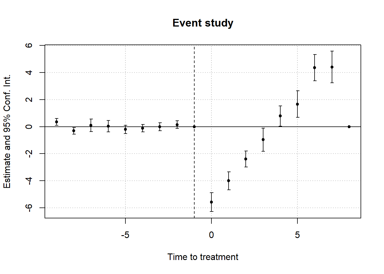
coefplot(est)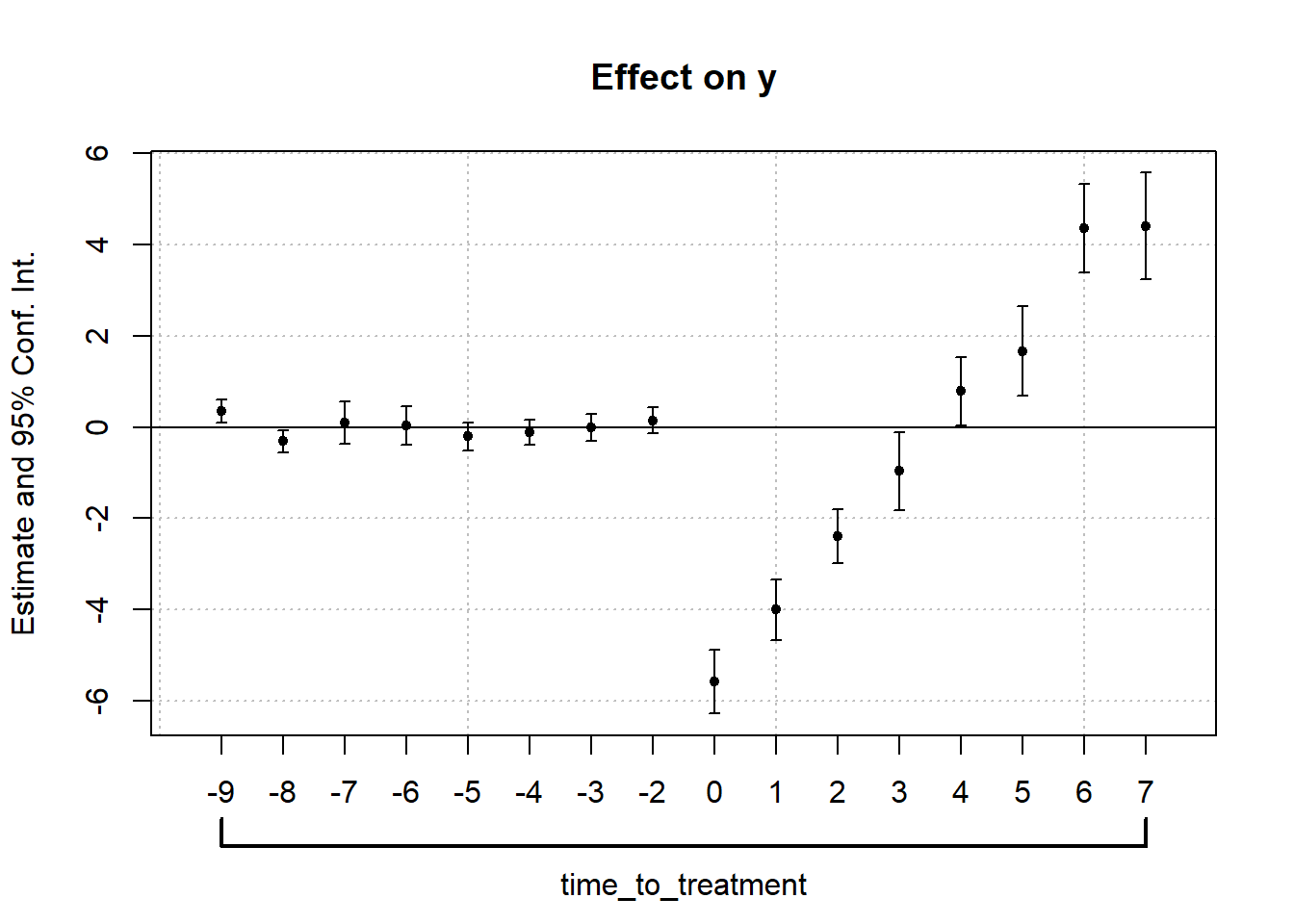

mult_est <- did2s::event_study(
    data = fixest::base_stagg |>
        dplyr::mutate(year_treated = dplyr::if_else(year_treated == 10000, 0, year_treated)),
    gname = "year_treated",
    idname = "id",
    tname = "year",
    yname = "y",
    estimator = "all"
)
#> Error in purrr::map(., function(y) { : ℹ In index: 1.
#> ℹ With name: y.
#> Caused by error in `.subset2()`:
#> ! no such index at level 1
did2s::plot_event_study(mult_est)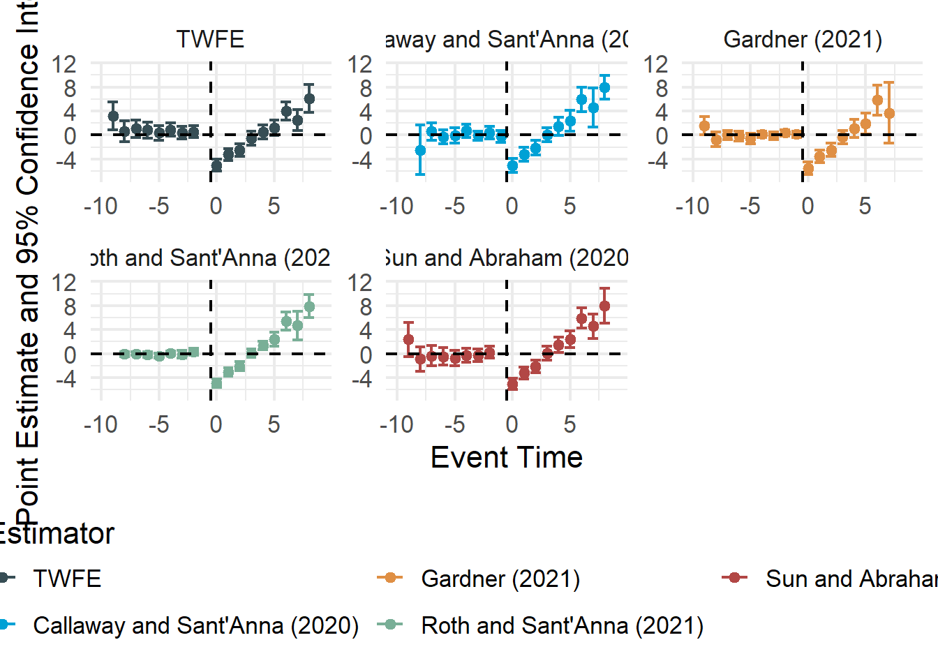

Borusyak et al. (2024) didimputation

This version is currently not working

library(didimputation)
library(fixest)
data("base_stagg")

did_imputation(
    data = base_stagg,
    yname = "y",
    gname = "year_treated",
    tname = "year",
    idname = "id"
)

---

35.12.8 Reshaped Inverse Probability Weighting - TWFE Estimator

The Reshaped Inverse Probability Weighting (RIPW) estimator extends the classic TWFE regression framework to account for arbitrary, time- and unit-varying treatment assignment mechanisms. This approach leverages an explicit model for treatment assignment to achieve design robustness, maintaining consistency even when traditional fixed-effects outcome models are misspecified.

The RIPW-TWFE framework is particularly relevant in panel data settings with general treatment patterns

• staggered adoption

• transient treatments.

---

Setting and Notation

• Panel data with \(n\) units observed over \(T\) time periods.

• Potential outcomes: For each unit \(i \in \{1, \dots, n\}\) and time \(t \in \{1, \dots, T\}\):

  \[ Y_{it}(1), \quad Y_{it}(0) \]

• Observed outcomes:

  \[ Y_{it} = W_{it} Y_{it}(1) + (1 - W_{it}) Y_{it}(0) \]

• Treatment assignment path for unit \(i\):

  \[ \mathbf{W}_i = (W_{i1}, \dots, W_{iT}) \in {0,1}^T \]

• Generalized Propensity Score (GPS): For unit \(i\), the probability distribution over treatment paths:

  \[ \mathbf{W}_i \sim \pi_i(\cdot) \]

  where \(\pi_i(w)\) is known or estimated.

---

Assumptions

1. Binary Treatment: \(W_{it} \in {0,1}\) for all \(i\) and \(t\).

2. No Dynamic Effects: Current outcomes depend only on current treatment, not past treatments.

3. Overlap Condition (Assumption 2.2 from Arkhangelsky et al. (2024)):

   There exists a subset \(S^* \subseteq \{0,1\}^T\), with \(|S^*| \ge 2\) and \(S^* \not\subseteq \{0_T, 1_T\}\), such that:

   \[ \pi_i(w) > c > 0, \quad \forall w \in S^*, \forall i \in \{1, \dots, n\} \]

4. Maximal Correlation Decay (Assumption 2.1): Dependence between units decays at rate \(n^{-q}\) for some \(q \in (0,1]\).

5. Bounded Second Moments (Assumption 2.3): \(\sup_{i,t,w} \mathbb{E}[Y_{it}^2(w)] < M < \infty\).

---

Key Quantities of Interest

• Unit-Time Specific Treatment Effect:

  \[ \tau_{it} = Y_{it}(1) - Y_{it}(0) \]

• Time-Specific Average Treatment Effect:

  \[ \tau_t = \frac{1}{n} \sum_{i=1}^n \tau_{it} \]

• Doubly Averaged Treatment Effect (DATE):

  \[ \tau(\xi) = \sum_{t=1}^T \xi_t \tau_t = \sum_{t=1}^T \xi_t \left( \frac{1}{n} \sum_{i=1}^n \tau_{it} \right) \]

  where \(\xi = (\xi_1, \dots, \xi_T)\) is a vector of non-negative weights such that \(\sum_{t=1}^T \xi_t = 1\).

• Special Case: Equally weighted DATE:

  \[ \tau_{\text{eq}} = \frac{1}{nT} \sum_{t=1}^T \sum_{i=1}^n \tau_{it} \]

---

Inverse Probability Weighting (IPW) methods are widely used to correct for selection bias in treatment assignment by reweighting observations according to their probability of receiving a given treatment. In panel data settings with TWFE regression, the IPW approach can be incorporated to address non-random treatment assignments over time and across units.

We begin with the classic TWFE regression objective, then show how IPW modifies it, and finally generalize to the Reshaped IPW (RIPW) estimator.

---

The unweighted TWFE estimator minimizes the following objective function:

\[ \min_{\tau, \mu, \{\alpha_i\}, \{\lambda_t\}} \sum_{i=1}^{n} \sum_{t=1}^{T} \left( Y_{it} - \mu - \alpha_i - \lambda_t - W_{it} \tau \right)^2 \]

where

• \(n\): Total number of units (e.g., individuals, firms, regions).
• \(T\): Total number of time periods.
• \(Y_{it}\): Observed outcome for unit \(i\) at time \(t\).
• \(W_{it}\): Binary treatment indicator for unit \(i\) at time \(t\).
  • \(W_{it} = 1\) if unit \(i\) is treated at time \(t\); \(0\) otherwise.
• \(\tau\): Parameter of interest, representing the Average Treatment Effect under the TWFE model.
• \(\mu\): Common intercept, capturing the overall average outcome level across all units and times.
• \(\alpha_i\): Unit-specific fixed effects, controlling for time-invariant heterogeneity across units.
• \(\lambda_t\): Time-specific fixed effects, controlling for shocks or common trends that affect all units in time period \(t\).

This standard TWFE regression assumes parallel trends across units in the absence of treatment and ignores the treatment assignment mechanism.

---

The IPW-TWFE estimator modifies the classic TWFE regression by reweighting the contribution of each observation according to the inverse probability of the entire treatment path for unit \(i\).

The weighted objective function is:

\[ \min_{\tau, \mu, \{\alpha_i\}, \{\lambda_t\}} \sum_{i=1}^{n} \sum_{t=1}^{T} \left( Y_{it} - \mu - \alpha_i - \lambda_t - W_{it} \tau \right)^2 \cdot \frac{1}{\pi_i(\mathbf{W}_i)} \]

where

• \(\pi_i(\mathbf{W}_i)\): The generalized propensity score (GPS) for unit \(i\).
  • This is the joint probability that unit \(i\) follows the entire treatment assignment path \(\mathbf{W}_i = (W_{i1}, W_{i2}, \dots, W_{iT})\).
  • It represents the assignment mechanism, which may be known (in experimental designs) or estimated (in observational studies).

By weighting the squared residual for each unit-time observation by \(\frac{1}{\pi_i(\mathbf{W}_i)}\), the IPW-TWFE estimator adjusts for non-random treatment assignment, similar to the role of IPW in cross-sectional data.

---

The Reshaped IPW (RIPW) estimator further generalizes the IPW approach by introducing a user-specified reshaped design distribution, denoted by \(\Pi\), over the space of treatment assignment paths.

The RIPW-TWFE estimator minimizes the following weighted objective:

\[ \hat{\tau}_{RIPW}(\Pi) = \arg \min_{\tau, \mu, \{\alpha_i\}, \{\lambda_t\}} \sum_{i=1}^{n} \sum_{t=1}^{T} \left( Y_{it} - \mu - \alpha_i - \lambda_t - W_{it} \tau \right)^2 \cdot \frac{\Pi(\mathbf{W}_i)}{\pi_i(\mathbf{W}_i)} \]

where

• \(\Pi(\mathbf{W}_i)\): A user-specified reshaped distribution over the treatment assignment paths \(\mathbf{W}_i\).
  • It describes an alternative “design” the researcher wants to emulate, possibly reflecting hypothetical or target assignment mechanisms.
• The weight \(\frac{\Pi(\mathbf{W}_i)}{\pi_i(\mathbf{W}_i)}\) can be interpreted as a likelihood ratio:
  • If \(\pi_i(\cdot)\) is the true assignment distribution, reweighting by \(\Pi(\cdot)\) effectively shifts the sampling design from \(\pi_i\) to \(\Pi\).
• The ratio \(\frac{\Pi(\mathbf{W}_i)}{\pi_i(\mathbf{W}_i)}\) adjusts for differences between the observed assignment mechanism and the target design.

---

Support of \(\mathbf{W}_i\)

The support of the treatment assignment paths is defined as:

\[ \mathbb{S} = \bigcup_{i=1}^{n} \text{Supp}(\mathbf{W}_i) \]

• \(\text{Supp}(\mathbf{W}_i)\): The support of the random variable \(\mathbf{W}_i\), i.e., the set of all treatment paths with positive probability under \(\pi_i(\cdot)\).
• \(\mathbb{S}\) represents the combined support across all units \(i = 1, \dots, n\).
• \(\Pi(\cdot)\) should have support contained within \(\mathbb{S}\), to ensure valid reweighting.

---

Special Cases of the RIPW Estimator

The choice of \(\Pi(\cdot)\) determines the behavior and interpretation of the RIPW estimator. Several special cases are noteworthy:

• Uniform Reshaped Design:

  \[ \Pi(\cdot) \sim \text{Uniform}(\mathbb{S}) \]

  • Here, \(\Pi\) places equal probability mass on each possible treatment path in \(\mathbb{S}\).

  • The weight becomes:

    \[ \frac{\Pi(\mathbf{W}_i)}{\pi_i(\mathbf{W}_i)} = \frac{1 / |\mathbb{S}|}{\pi_i(\mathbf{W}_i)} \]

  • This reduces RIPW to the standard IPW-TWFE estimator, in which the target is a uniform treatment assignment design.

• Reshaped Design Equals True Assignment:

  \[ \Pi(\cdot) = \pi_i(\cdot) \]

  • The weight simplifies to:

    \[ \frac{\Pi(\mathbf{W}_i)}{\pi_i(\mathbf{W}_i)} = 1 \]

  • The RIPW estimator reduces to the unweighted TWFE regression, consistent with an experiment where the assignment mechanism \(\pi_i\) is known and correctly specified.

---

To ensure that \(\hat{\tau}_{RIPW}(\Pi)\) consistently estimates the DATE \(\tau(\xi)\), we solve the DATE Equation:

\[ \mathbb{E}_{\mathbf{W} \sim \Pi} \left[ \left( \text{diag}(\mathbf{W}) - \xi \mathbf{W}^\top \right) J \left( \mathbf{W} - \mathbb{E}_{\Pi}[\mathbf{W}] \right) \right] = 0 \]

• \(J = I_T - \frac{1}{T} \mathbf{1}_T \mathbf{1}_T^\top\) is a projection matrix removing the mean.
• Solving this equation ensures consistency of the RIPW estimator for \(\tau(\xi)\).

---

Choosing the Reshaped Distribution \(\Pi\)

• If the support \(\mathbb{S}\) and \(\pi_i(\cdot)\) are known, \(\Pi\) can be specified directly.
• Closed-form solutions for \(\Pi\) are available in settings such as staggered adoption designs.
• When closed-form solutions are unavailable, optimization algorithms (e.g., BFGS) can be employed to solve the DATE equation numerically.

---

Properties

• The RIPW estimator provides design-robustness:
  • It can correct for misspecified outcome models by properly reweighting according to the assignment mechanism.
  • It accommodates complex treatment assignment processes, such as staggered adoption and non-random assignment.
• The flexibility to choose \(\Pi(\cdot)\) allows researchers to target estimands that represent specific policy interventions or hypothetical designs.

The RIPW estimator has a double robustness property:

• \(\hat{\tau}_{RIPW}(\Pi)\) is consistent if either:

  • The assignment model \(\pi_i(\cdot)\) is correctly specified or

  • The outcome regression (TWFE) model is correctly specified.

This feature is particularly valuable in quasi-experimental designs where the parallel trends assumption may not hold globally.

• Design-Robustness: RIPW corrects for negative weighting issues identified in the TWFE literature (e.g., Goodman-Bacon (2021); De Chaisemartin and D’haultfœuille (2023)).
• Unlike conventional TWFE regressions, which can yield biased estimands under heterogeneity, RIPW explicitly targets user-specified weighted averages (DATE).
• In randomized experiments, RIPW ensures the effective estimand is interpretable as a population-level average, determined by the design \(\Pi\).

---

35.12.9 Dynamic Treatment Effect Estimation with Interactive Fixed Effects and Short Panels

Brown and Butts (2025)

---

35.12.10 Switching Difference-in-Differences Estimator (De Chaisemartin and d’Haultfoeuille 2020)

TWFE hinges on restrictive assumptions (e.g., the homogeneity of treatment effects across time and groups). When this assumption is violated, TWFE can yield misleading results, including estimates with signs opposite to all underlying effects.

We consider a standard panel data setup with \(G\) groups and \(T\) time periods. Each observation belongs to a group-period cell \((g, t)\), and treatment \(D_{g,t} \in {0,1}\) is assigned at the group-time level.

Let \(Y_{i,g,t}\) be the outcome of individual \(i\) in group \(g\) at time \(t\), with potential outcomes \(Y_{i,g,t}(1)\) and \(Y_{i,g,t}(0)\). Observed outcomes satisfy:

\[ Y_{i,g,t} = D_{g,t} \cdot Y_{i,g,t}(1) + (1 - D_{g,t}) \cdot Y_{i,g,t}(0) \]

The canonical TWFE regression is:

\[ Y_{i,g,t} = \alpha_g + \lambda_t + \beta^{fe} D_{g,t} + \varepsilon_{i,g,t} \]

where \(\alpha_g\) are group fixed effects, \(\lambda_t\) are time fixed effects, and \(\beta^{fe}\) is interpreted as the treatment effect only under homogeneous treatment effects.

35.12.10.1 Heterogeneous Treatment Effects and Weighting Bias

When treatment effects vary across \((g,t)\) cells, the TWFE estimator \(\hat{\beta}^{fe}\) is no longer a simple average. Instead, it can be decomposed into a weighted sum of cell-specific average treatment effects:

\[ \beta^{fe} = \mathbb{E} \left[ \sum_{(g,t): D_{g,t}=1} w_{g,t} \Delta_{g,t} \right] \]

where:

• \(\Delta_{g,t} = \mathbb{E}[Y_{g,t}(1) - Y_{g,t}(0)]\) is the average treatment effect in cell \((g,t)\)
• \(w_{g,t}\) are weights that can be negative and sum to one.

Some weights are negative because TWFE implicitly compares outcomes across all treated and untreated groups, even when “controls” are themselves treated. These comparisons can subtract out treatment effects, leading to negative weights.

---

35.12.10.2 Illustration: Negative Weights Can Flip Signs

For example, suppose:

• Group 1 is treated only in period 3: \(\Delta_{1,3} = 1\)
• Group 2 is treated in periods 2 and 3:
  • \(\Delta_{2,2} = 1\)
  • \(\Delta_{2,3} = 4\)

Then TWFE produces:

\[ \beta^{fe} = \frac{1}{2} \Delta_{1,3} + \Delta_{2,2} - \frac{1}{2} \Delta_{2,3} = \frac{1}{2} + 1 - 2 = -0.5 \]

All \(\Delta_{g,t}\)s are positive, but the TWFE estimate is negative.

---

To assess the extent to which TWFE may be misleading, compute the robustness ratio:

\[ \sigma^{fe}_\_ = \frac{|\hat{\beta}^{fe}|}{\hat{\sigma}(w)} \]

Where:

• \(\hat{\sigma}(w)\) is the standard deviation of the TWFE weights across treated cells.
• A small \(\sigma^{fe}_\_\) indicates that minor heterogeneity can reverse the sign of the estimate.

This can be estimated directly from data and helps determine whether TWFE is reliable in your context.

---

35.12.10.3 DID_M Estimator: A Robust Alternative

De Chaisemartin and d’Haultfoeuille (2020) propose the DID_M estimator, which is valid under heterogeneous treatment effects. It focuses only on switching groups, using non-switchers as controls in a local difference-in-differences design.

Let \(S\) denote the set of all \((g,t)\) cells where treatment status changes between \(t-1\) and \(t\). The DID_M estimator is:

\[ \text{DID}_M = \sum_{t=2}^{T} \left( \frac{N_{1,0,t}}{N_S} \cdot \text{DID}^+_t + \frac{N_{0,1,t}}{N_S} \cdot \text{DID}^-_t \right) \]

Where:

• \(\text{DID}^+_t\) compares joiners to stable untreated groups
• \(\text{DID}^-_t\) compares leavers to stable treated groups
• \(N_S\) is the total number of observations in switching cells

DID_M requires:

1. Common trends for both treated and untreated potential outcomes
2. Existence of stable groups at every \(t\) (i.e., some groups don’t change treatment status)
3. No Ashenfelter dip (treatment not triggered by negative shocks)

These assumptions are weaker than those required for TWFE to be unbiased.

De Chaisemartin and d’Haultfoeuille (2020) also propose a placebo version of DID_M using pre-treatment periods. If pre-treatment differences exist between switchers and non-switchers, this indicates violation of the parallel trends assumption. This test is analogous to pre-trend checks in event-study designs.

# Load required packages
library(fixest)            # For TWFE model and dataset
library(TwoWayFEWeights)   # For decomposing TWFE weights
library(DIDmultiplegt)     # For robust SDID estimator

# Load the sample staggered adoption dataset
data("base_stagg")

# Preview the data
head(base_stagg)
#>   id year year_treated time_to_treatment treated treatment_effect_true
#> 2 90    1            2                -1       1                     0
#> 3 89    1            3                -2       1                     0
#> 4 88    1            4                -3       1                     0
#> 5 87    1            5                -4       1                     0
#> 6 86    1            6                -5       1                     0
#> 7 85    1            7                -6       1                     0
#>           x1           y
#> 2 -1.0947021  0.01722971
#> 3 -3.7100676 -4.58084528
#> 4  2.5274402  2.73817174
#> 5 -0.7204263 -0.65103066
#> 6 -3.6711678 -5.33381664
#> 7 -0.3152137  0.49562631

35.12.10.3.1 Estimate TWFE Model

# Run standard TWFE using fixest
twfe <- feols(y ~ treatment | id + year,
                    data = base_stagg |>
                        dplyr::mutate(treatment = dplyr::if_else(time_to_treatment < 0, 0, 1)))
summary(twfe)
#> OLS estimation, Dep. Var.: y
#> Observations: 950
#> Fixed-effects: id: 95,  year: 10
#> Standard-errors: IID 
#>           Estimate Std. Error t value  Pr(>|t|)    
#> treatment -3.46761   0.336041 -10.319 < 2.2e-16 ***
#> ---
#> Signif. codes:  0 '***' 0.001 '**' 0.01 '*' 0.05 '.' 0.1 ' ' 1
#> RMSE: 2.471     Adj. R2: 0.272265
#>               Within R2: 0.111912

35.12.10.3.2 Decompose Weights with TwoWayFEWeights

twfe_weights <- twowayfeweights(
    data = base_stagg |> dplyr::mutate(treatment = dplyr::if_else(time_to_treatment < 0, 0, 1)),
    Y = "y",
    G = "year_treated",
    T = "year",
    D = "treatment", 
    summary_measures = T
)

# Show summary
twfe_weights
#> 
#> Under the common trends assumption,
#> the TWFE coefficient beta, equal to -3.4676, estimates a weighted sum of 45 ATTs.
#> 41 ATTs receive a positive weight, and 4 receive a negative weight.
#> 
#> ────────────────────────────────────────── 
#> Treat. var: treatment    ATTs    Σ weights 
#> ────────────────────────────────────────── 
#> Positive weights           41       1.0238 
#> Negative weights            4      -0.0238 
#> ────────────────────────────────────────── 
#> Total                      45            1 
#> ──────────────────────────────────────────
#> 
#> Summary Measures:
#>   TWFE Coefficient (β_fe): -3.4676
#>   min σ(Δ) compatible with β_fe and Δ_TR = 0: 4.8357
#>   min σ(Δ) compatible with treatment effect of opposite sign than β_fe in all (g,t) cells: 36.1549
#>   Reference: Corollary 1, de Chaisemartin, C and D'Haultfoeuille, X (2020a)
#> 
#> The development of this package was funded by the European Union (ERC, REALLYCREDIBLE,GA N. 101043899).

35.12.10.3.3 Estimate DID_M (Switching DID Estimator) with DIDmultiplegt

# Estimate robust SDID estimator (DID_M)
did_m <- did_multiplegt(
        mode = "dyn",
        df = base_stagg |>
            dplyr::mutate(treatment = dplyr::if_else(time_to_treatment < 0, 0, 1)),
        outcome = "y",
        group = "year_treated",
        time = "year",
        treatment = "treatment",
        effects = 5,
        # controls = c("x1"),
        placebo = 2
    )

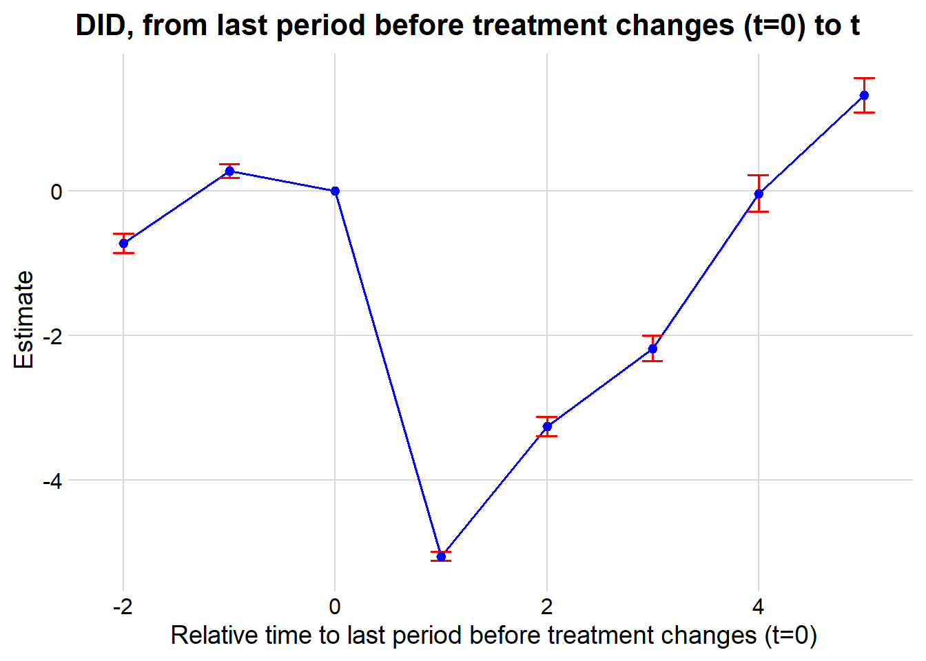
summary(did_m)
#> 
#> ----------------------------------------------------------------------
#>        Estimation of treatment effects: Event-study effects
#> ----------------------------------------------------------------------
#>              Estimate SE      LB CI    UB CI    N  Switchers
#> Effect_1     -5.04943 0.03256 -5.11324 -4.98562 54 9        
#> Effect_2     -3.25734 0.06712 -3.38889 -3.12579 44 8        
#> Effect_3     -2.17826 0.08866 -2.35204 -2.00449 35 7        
#> Effect_4     -0.03749 0.12841 -0.28916 0.21418  27 6        
#> Effect_5     1.31986  0.12128 1.08216  1.55756  20 5        
#> 
#> Test of joint nullity of the effects : p-value = 0.0000
#> ----------------------------------------------------------------------
#>     Average cumulative (total) effect per treatment unit
#> ----------------------------------------------------------------------
#>  Estimate        SE     LB CI     UB CI         N Switchers 
#>  -2.29649   0.07360  -2.44074  -2.15223        80        35 
#> Average number of time periods over which a treatment effect is accumulated: 2.7143
#> 
#> ----------------------------------------------------------------------
#>      Testing the parallel trends and no anticipation assumptions
#> ----------------------------------------------------------------------
#>              Estimate SE      LB CI    UB CI    N  Switchers
#> Placebo_1    0.27204  0.04917 0.17567  0.36841  44 8        
#> Placebo_2    -0.72910 0.06790 -0.86219 -0.59601 27 6        
#> 
#> Test of joint nullity of the placebos : p-value = 0.0000
#> 
#> 
#> The development of this package was funded by the European Union.
#> ERC REALLYCREDIBLE - GA N. 101043899

---

35.12.11 Augmented/Forward DID

• DID Methods for Limited Pre-Treatment Periods (see Table 35.11):

Table 35.11: Augmented DID and Forward DID for settings with few pre-treatment periods, contrasted on scenario and approach.

Method	Scenario	Approach
Augmented DID (Li and Van den Bulte 2023)	Treatment outcome is outside the range of control units	Constructs the treatment counterfactual using a scaled average of control units
Forward DID (Li 2024)	Treatment outcome is within the range of control units	Uses a forward selection algorithm to choose relevant control units before applying DID

---

35.12.12 Doubly Robust Difference-in-Differences Estimators

In its simplest “canonical” form, DID compares the before-and-after outcomes of one group that eventually receives a treatment (the “treated” group) with the before-and-after outcomes of another group that never receives the treatment (the “comparison” group). Under the parallel trends assumption, DID can recover the average treatment effect on the treated (ATT).

Practitioners often enrich DID analyses by conditioning on observed covariates to mitigate violations of the unconditional parallel trends assumption. Once conditioning on covariates, the DID framework remains attractive, provided that conditional parallel trends hold.

Historically, two main approaches have emerged for DID estimation in the presence of covariates:

1. Outcome Regression (OR) (Heckman et al. 1997). Model the outcome evolution for the comparison group (and possibly for the treated group), and then plug these fitted outcome equations into the DID formula.
2. Inverse Probability Weighting (IPW) (Abadie 2005). Model the probability of treatment conditional on covariates (the “propensity score”) and use inverse-probability reweighting to reconstruct appropriate counterfactuals for the treated group.

A key insight in semiparametric causal inference is that one can combine these two approaches (modeling the outcome regression and the propensity score in tandem) to form an estimator that remains consistent if either the outcome-regression equations are correctly specified or the propensity-score equation is correctly specified. Such an estimator is called doubly robust (Sant’Anna and Zhao 2020).

This section covers both cases of (i) panel data (where we observe each unit in both pre- and post-treatment periods) and (ii) repeated cross-section data (where, in each period, we observe a new random sample of units).

Under suitable conditions, the proposed doubly robust estimators not only exhibit desirable robustness properties to misspecification but can also attain the semiparametric efficiency bound, making them locally efficient if all working models are correct.

---

35.12.12.1 Notation and set-up

• Two-time-period design. We consider a setting with two time periods: \(t = 0\) (pre-treatment) and \(t = 1\) (post-treatment). A subset of units receives the treatment only at \(t = 1\). Hence for a unit \(i\):

  • \(D_i = D_{i1} \in {0, 1}\) is an indicator for receiving treatment by time 1 (so \(D_{i0} = 0\) for all \(i\)).
  • \(Y_{it}\) is the observed outcome at time \(t\).

• Potential outcomes. We adopt the potential outcomes framework. Let \[ Y_{it}(1) = \text{potential outcome of unit }i \text{ at time } t \text{ if treated,} \] \[ Y_{it}(0) = \text{potential outcome of unit }i \text{ at time } t \text{ if not treated.} \] Then the observed outcome satisfies \(Y_{it} = D_i Y_{it}(1) + (1-D_i) Y_{it}(0)\).

• Covariates. A vector of observed pre-treatment covariates is denoted \(X_i\). Throughout, we assume the first component of \(X_i\) is a constant (intercept).

• Data structures.

  1. Panel data. We observe \(\{(Y_{i0}, Y_{i1}, D_i, X_i)\}_{i=1}^n\), a sample of size \(n\) drawn i.i.d. from an underlying population.
  2. Repeated cross-sections. In period \(t\), we observe a fresh random sample of units. Let \(T_i\in {0,1}\) be an indicator for whether an observation is drawn in the post-treatment period \((T_i=1)\) or the pre-treatment period \((T_i=0)\). Write \(\{(Y_i, D_i, X_i, T_i)\}_{i=1}^n\). Here, if \(T_i=1\), then \(Y_i \equiv Y_{i1}\); if \(T_i=0\), then \(Y_i \equiv Y_{i0}\). We typically assume a stationarity condition, namely that the distribution of \((D, X)\) is stable across the two periods.

Let \(n_1\) and \(n_0\) be the respective sample sizes for the post- and pre-treatment periods, so \(n_1 + n_0 = n\). Often we let \(\lambda = P(T=1)\approx n_1/n.\)

The focus is on the ATT: \[ \tau = \mathbb{E}[Y_{i1}(1) - Y_{i1}(0)\big| D_i=1]. \] Because we only observe \(Y_{i1}(1)\) for the treated group, the central challenge is to recover \(\mathbb{E}[Y_{i1}(0)\mid D_i=1]\). Under standard DID assumptions, we identify \(\tau\) by comparing the treated group’s evolution in outcomes to the comparison group’s evolution in outcomes.

We require two key assumptions:

1. Conditional parallel trends
   For \(t=0,1\), let \[ \mathbb{E}[Y_{1}(0) - Y_{0}(0)\mid D=1, X] = \mathbb{E}[Y_{1}(0) - Y_{0}(0)\mid D=0, X]. \] This means that, conditional on \(X\), in the absence of treatment, the treated and comparison groups would have had parallel outcome evolutions.

2. Overlap
   There exists \(\varepsilon>0\) such that \[ \varepsilon \le P(D=1\vert X)\le 1-\varepsilon \] That is, we require that a nontrivial fraction of the population is treated, and for each \(X\), there is a nontrivial probability of being in the untreated group (\(D=0\)).

Under these assumptions, we can identify \(\mathbb{E}[Y_{1}(0)\mid D=1]\) in a semiparametric fashion, either by modeling the outcome regressions (the OR approach) or by modeling the propensity score (the IPW approach).

---

35.12.12.2 Two Traditional DID Approaches

We briefly outline the classical DID estimators that rely solely on either outcome regressions or inverse probability weighting, to motivate the doubly robust idea.

35.12.12.2.1 Outcome-regression (OR) approach

Define

\[ m_{d,t}(x) = \mathbb{E}[Y_t \mid D=d, X=x]. \]

Under the conditional parallel trends assumption,

\[ \mathbb{E}[Y_{1}(0)\mid D=1 ] = \mathbb{E}[Y_{0}(0)\mid D=1] + \mathbb{E}[m_{0,1}(X) - m_{0,0}(X)\big\vert D=1]. \]

Hence an OR-based DID estimator (for panel or repeated cross-section) typically looks like

\[ \hat{\tau}^{\mathrm{reg}} = \overline{Y}_{1,1} - \left(\overline{Y}_{1,0} + \frac{1}{n_{\mathrm{treat}}} \sum_{i:D_i=1} [ \hat{m}_{0,1}(X_i) - \hat{m}_{0,0}(X_i) ] \right), \]

where \(\overline{Y}_{d,t}\) is the sample mean of \(Y_t\) among units with \(D=d\), and \(\hat{m}_{0,t}\) is some fitted model (e.g., linear or semiparametric) for \(\mathbb{E}[Y_t \mid D=0,X]\).

This OR estimator is consistent if (and only if) we have correctly specified the two outcome-regression functions \(m_{0,1}(x)\) and \(m_{0,0}(x)\). If these regressions are misspecified, the estimator will generally be biased.

35.12.12.2.2 IPW approach

An alternative is to model the propensity score

\[ p(x)= P(D=1 \mid X=x), \]

and use a Horvitz–Thompson-type reweighting (Horvitz and Thompson 1952) to reconstruct what “would have happened” to the treated group under no treatment. In the panel-data case, Abadie (2005) show that the ATT can be identified via

\[ \tau = \frac{1}{\mathbb{E}[D]} \mathbb{E}\left[ \frac{D - p(X)}{1 - p(X)} (Y_1 - Y_0) \right] \]

Hence an IPW estimator for panel data is

\[ \hat{\tau}^{\mathrm{ipw,p}} = \frac{1}{\overline{D}} \sum_{i=1}^n \left[\frac{D_i - \hat{p}(X_i)}{1-\hat{p}(X_i)}\right] \frac{1}{n}(Y_{i1} - Y_{i0}), \]

where \(\hat{p}(\cdot)\) is a fitted propensity score model. Similar expressions exist for repeated cross-sections, with small modifications to handle the fact that we observe \(Y_1\) only if \(T=1\), etc.

This IPW estimator is consistent if (and only if) the propensity score is correctly specified, i.e., \(\hat{p}(x)\approx p(x)\). If the propensity-score model is incorrect, the estimator may be severely biased.

---

35.12.12.3 Doubly Robust DID: Main Identification

The doubly robust (DR) idea is to combine the OR and IPW approaches so that the resulting estimator is consistent if either the OR model is correct or the propensity-score model is correct. Formally, consider two generic “working” models:

• \(\pi(X)\) for \(p(X)\), i.e., a model for the propensity score,

• \(\mu_{0,t}(X)\) for the outcome regressions \(m_{0,t}(X)=\mathbb{E}[Y_t \mid D=0,X]\).

We define two “DR moments” for each data structure.

35.12.12.3.1 DR estimand for panel data

When panel data are available, define

\[ \Delta Y = Y_1 - Y_0, \quad \mu_{0,\Delta}(X)=\mu_{0,1}(X)-\mu_{0,0}(X). \]

Then a DR moment for \(\tau\) is:

\[ \tau^{\mathrm{dr,p}} = \mathbb{E}\left[ \left(w_{1}^{\mathrm{p}}(D)-w_{0}^{\mathrm{p}}(D,X;\pi)\right) \left(\Delta Y -\mu_{0,\Delta}(X)\right) \right] \]

where

\[ w_{1}^{\mathrm{p}}(D)=\frac{D}{\mathbb{E}[D]}, \quad\quad w_{0}^{\mathrm{p}}(D,X;\pi)=\frac{\pi(X)(1-D)}{(1-\pi(X))\mathbb{E}[\tfrac{\pi(X)(1-D)}{1-\pi(X)}]}. \]

It can be shown that \(\tau^{\mathrm{dr,p}} = \tau\) provided either \(\pi(x)=p(x)\) almost surely (a.s.) or \(\mu_{0,\Delta}(x)=m_{0,\Delta}(x)\) a.s. (the latter meaning that at least the regression for the comparison group is correct).

35.12.12.3.2 DR estimands for repeated cross-sections

When we only have repeated cross-sections, the DR construction must account for the fact that \(Y_0, Y_1\) are not observed jointly on the same individuals. Let \(\lambda = P(T=1)\). Then two valid DR estimands are:

1. \[ \tau^{\mathrm{dr,rc}}_{1} = \mathbb{E}\left[(w_{1}^{\mathrm{rc}}(D,T)-w_{0}^{\mathrm{rc}}(D,T,X;\pi))(Y -\mu_{0,Y}(T,X))\right], \] where \[ w_{1}^{\mathrm{rc}}(D,T) = \frac{D1{T=1}} {\mathbb{E}[D1{T=1}]} - \frac{D1{T=0}} {\mathbb{E}[D1{T=0}]}, \] and \[ w_{0}^{\mathrm{rc}}(D,T,X;\pi) = \frac{\pi(X)(1-D)1{T=1}}{(1-\pi(X))\mathbb{E}[\tfrac{\pi(X)(1-D)1{T=1}}{(1-\pi(X))}]} - \frac{\pi(X)(1-D)1{T=0}}{(1-\pi(X))\mathbb{E}[\tfrac{\pi(X)(1-D)1{T=0}}{(1-\pi(X))}]}, \] and \(\mu_{0,Y}(T,X)=T\cdot\mu_{0,1}(X)+(1-T)\cdot\mu_{0,0}(X)\).

2. \[ \begin{aligned} \tau^{\mathrm{dr,rc}}_{2} ={}& \tau^{\mathrm{dr,rc}}_{1} \\ &+ \left[\mathbb{E}(\mu_{1,1}(X) - \mu_{0,1}(X)|D=1) - \mathbb{E}(\mu_{1,1}(X) - \mu_{0,1}(X)|D=1,T=1)\right] \\ &- \left[\mathbb{E}(\mu_{1,0}(X) - \mu_{0,0}(X)|D=1) - \mathbb{E}(\mu_{1,0}(X) - \mu_{0,0}(X)|D=1,T=0)\right] \end{aligned} \] where \(\mu_{d,t}(x)\) is a model for \(m_{d,t}(x)=\mathbb{E}[Y \mid D=d,T=t,X=x]\).

One can show \(\tau^{\mathrm{dr,rc}}_1 = \tau^{\mathrm{dr,rc}}_2 = \tau\) as long as the stationarity of \((D,X)\) across time holds and either the propensity score model \(\pi(x)=p(x)\) is correct or the comparison-group outcome regressions are correct (Sant’Anna and Zhao 2020). Notably, \(\tau^{\mathrm{dr,rc}}_2\) also includes explicit modeling of the treated group’s outcomes. However, in terms of identification alone, \(\tau^{\mathrm{dr,rc}}_1\) and \(\tau^{\mathrm{dr,rc}}_2\) share the same double-robust property.

---

35.12.12.4 Semiparametric Efficiency Bounds and Local Efficiency

An important concept in semiparametric inference is the semiparametric efficiency bound, which is the infimum of the asymptotic variance across all regular estimators that exploit only the imposed assumptions (parallel trends, overlap, stationarity). Equivalently, one can think of it as the variance of the “efficient influence function” (EIF).

We highlight key results:

1. Efficient influence function for panel data

Under the above mentioned assumptions (i.i.d. data generating process, overlap, and conditional parallel trends) and without imposing further parametric constraints on \((m_{d,t},p)\), one can derive that the EIF for \(\tau\) in the panel-data setting is

\[ \begin{aligned} \eta^{e,\mathrm{p}}(Y_1, Y_0, D, X) &= \frac{D}{\mathbb{E}[D]}[m_{1,\Delta}(X) - m_{0,\Delta}(X) - \tau]\\ &\quad +\frac{D}{\mathbb{E}[D]}[\Delta Y - m_{1,\Delta}(X)]\\ &\quad -\frac{\pi(X)(1-D)}{(1 - \pi(X))\mathbb{E}[\tfrac{\pi(X)(1-D)}{1 - \pi(X)}]}[\Delta Y - m_{0,\Delta}(X)] \end{aligned} \]

where \(\Delta Y = Y_1 - Y_0\) and \(m_{d,\Delta}(X) \equiv m_{d,1}(X) - m_{d,0}(X)\).

The associated semiparametric efficiency bound is \[ \mathbb{E}[\eta^{e,\mathrm{p}}(Y_1,Y_0,D,X)^2]. \] It can be shown that a DR DID estimator can attain this bound if (1) the propensity score is correctly modeled, and (2) the comparison-group outcome regressions are correctly modeled.

2. Efficient influence function for repeated cross-sections

Similarly, when only repeated cross-sections are available, the EIF becomes

\[ \begin{aligned} \eta^{e,\mathrm{rc}}(Y,D,T,X) &= \frac{D}{\mathbb{E}[D]}[m_{1,\Delta}(X) - m_{0,\Delta}(X) - \tau]\\ &\quad +\left[w_{1,1}^{\mathrm{rc}}(D,T)(Y - m_{1,1}(X)) - w_{1,0}^{\mathrm{rc}}(D,T)(Y - m_{1,0}(X))\right]\\ &\quad -\left[w_{0,1}^{\mathrm{rc}}(D,T,X;p)(Y - m_{0,1}(X)) - w_{0,0}^{\mathrm{rc}}(D,T,X;p)(Y - m_{0,0}(X))\right] \end{aligned} \]

with \(m_{d,\Delta}(X)=m_{d,1}(X)-m_{d,0}(X)\). The resulting efficiency bound is \(\mathbb{E}[\eta^{e,\mathrm{rc}}(Y,D,T,X)^2]\).

One can further show that having access to panel data can be strictly more informative (i.e., yields a smaller semiparametric variance bound) than repeated cross-sections. This difference can grow if the pre- and post-treatment samples are highly unbalanced.

---

35.12.12.5 Construction of Doubly Robust DID Estimators

1. Generic two-step approach

Building upon the DR moment expressions, a natural approach to estimation is:

1. First-stage modeling (nuisance parameters).
   • Estimate \(\hat{\pi}(X)\) for the propensity score, e.g. via logistic regression or other parametric or semiparametric methods.
   • Estimate \(\hat{m}_{0,t}(X)\) for \(t=0,1\). One might also estimate \(\hat{m}_{1,t}(X)\) if using the second DR estimator for repeated cross-sections.
2. Plug into the DR moment.
   Replace \(p\) with \(\hat{\pi}\) and \(m_{d,t}\) with \(\hat{m}_{d,t}\) in the chosen DR formula (panel or repeated cross-sections).

Because these estimators are DR, if either the propensity score is well specified or the outcome regressions for the comparison group are well specified, consistency is assured.

2. Improving efficiency and inference: special parametric choices

It is sometimes desirable to construct DR DID estimators that are also “DR for inference,” meaning that the asymptotic variance does not depend on which portion of the model is correct. Achieving that typically requires carefully choosing first-stage estimators so that the extra “estimation effect” vanishes in the influence-function calculations. Concretely:

• Propensity score: Use a logistic regression (and a special inverse probability tilting estimator) proposed by Graham et al. (2012).
• Outcome regressions: Use linear regressions with specific weights (or with OLS for the treated group).

One then obtains:

• For panel data: \[ \hat{\tau}^{\mathrm{dr,p}}_{\mathrm{imp}} = \frac{1}{n} \sum_{i=1}^n \left[w_{1}^{\mathrm{p}}(D_i) - w_{0}^{\mathrm{p}}(D_i,X_i;\hat{\gamma}^{\mathrm{ipt}})\right] \left[(Y_{i1}-Y_{i0}) - \hat{\mu}^{\mathrm{lin,p}}_{0,\Delta}(X_i;\hat{\beta}^{\mathrm{wls,p}}_{0,\Delta})\right], \] where \(\hat{\gamma}^{\mathrm{ipt}}\) is the “inverse probability tilting” estimate for the logit propensity score, and \(\hat{\beta}^{\mathrm{wls,p}}_{0,\Delta}\) is a weighted least squares estimate for the difference regressions of the comparison group. Under suitable regularity conditions, this estimator:

  1. Remains consistent if either the logit model or the linear outcome model for \(\Delta Y\) in the control group is correct.

  2. Has an asymptotic distribution that does not depend on which model is correct (thus simplifying inference).

  3. Achieves the semiparametric efficiency bound if both models are correct.

• For repeated cross-sections, one can analogously use logistic-based tilting for the propensity score and weighted/ordinary least squares for the control/treated outcome regressions. The second DR estimator \(\hat{\tau}^{\mathrm{dr,rc}}_{2}\) that models the treated group’s outcomes as well can, under correct specification of all models, achieve local efficiency.

---

35.12.12.6 Large-Sample Properties

Assume mild regularity conditions for consistency and asymptotic normality (e.g., overlapping support, identifiability of the pseudo-true parameters for the first-step models, and suitable rates of convergence) (Sant’Anna and Zhao 2020).

1. Double Robust Consistency.
   Each proposed DR DID estimator is consistent for \(\tau\) if either (a) \(\hat{p}(X)\) is consistent for \(p(X)\), or (b) the relevant outcome regressions \(\hat{m}_{0,t}(X)\) are consistent for \(m_{0,t}(X)\). Thus, we say the estimator is doubly robust to misspecification.

2. Asymptotic Normality.
   \[ \sqrt{n}(\hat{\tau}^{\mathrm{dr}} - \tau ) \xrightarrow{d} N(0,\mathrm{Var}(\text{IF})), \] where \(\mathrm{Var}(\text{IF})\) depends on which part(s) of the nuisance models are consistently estimated. In general, one must account for the variance contribution of the first-stage estimation. But under certain special constructions (the “improved DR” approaches with inverse probability tilting and specialized weighting), the first-stage does not contribute additional variance, making inference simpler.

3. Local Semiparametric Efficiency.
   If both the propensity score model and the outcome-regression models are correct, the estimator’s influence function matches the efficient influence function, hence achieving the semiparametric efficiency bound. In repeated cross-sections, the DR estimator that also models the treated group’s outcomes (namely \(\tau^{\mathrm{dr,rc}}_2\)) is the one that can achieve local efficiency.

---

35.12.12.7 Practical Implementation

In practice, the recommended workflow is:

1. Specify (and estimate) a flexible working model for the propensity score. A logistic regression with the inverse-probability-tilting approach is often a good default, as it simplifies subsequent steps if one wants DR inference.
2. Model the outcome of the comparison group over time. For panel data, one can directly model \(\Delta Y\). For repeated cross-sections, one typically models \(\{m_{0,t}(X)\}_{t=0,1}\).
3. (Optional) Model the outcome of the treated group if seeking the local-efficiency version of DR DID in repeated cross-sections.
4. Form the DR DID estimator by plugging the fitted models from steps (1)–(3) into the chosen DR moment expression.

Inference can often be carried out by taking the empirical variance of the estimated influence function: \[ \hat{V} = \frac{1}{n}\sum_{i=1}^n \hat{\eta}_i^2, \] where \(\hat{\eta}_i\) is the evaluator’s best estimate of the influence function for observation \(i\). Under certain “improved DR” constructions, the same \(\hat{\eta}_i\) works regardless of which part of the model is correct.

---

data('base_stagg')

library(did)

drdid_result <- att_gt(
    yname = "y",
    tname = "year",
    idname = "id",
    gname = "year_treated",
    xformla = ~ x1,
    data = base_stagg
)


aggte(drdid_result, type = "simple")
#> 
#> Call:
#> aggte(MP = drdid_result, type = "simple")
#> 
#> Reference: Callaway, Brantly and Pedro H.C. Sant'Anna.  "Difference-in-Differences with Multiple Time Periods." Journal of Econometrics, Vol. 225, No. 2, pp. 200-230, 2021. <https://doi.org/10.1016/j.jeconom.2020.12.001>, <https://arxiv.org/abs/1803.09015> 
#> 
#> 
#>      ATT    Std. Error     [ 95%  Conf. Int.] 
#>  -0.8636        0.5924    -2.0247      0.2974 
#> 
#> 
#> ---
#> Signif. codes: `*' confidence band does not cover 0
#> 
#> Control Group:  Never Treated,  Anticipation Periods:  0
#> Estimation Method:  Doubly Robust
agg.es <- aggte(drdid_result, type = "dynamic")

ggdid(agg.es)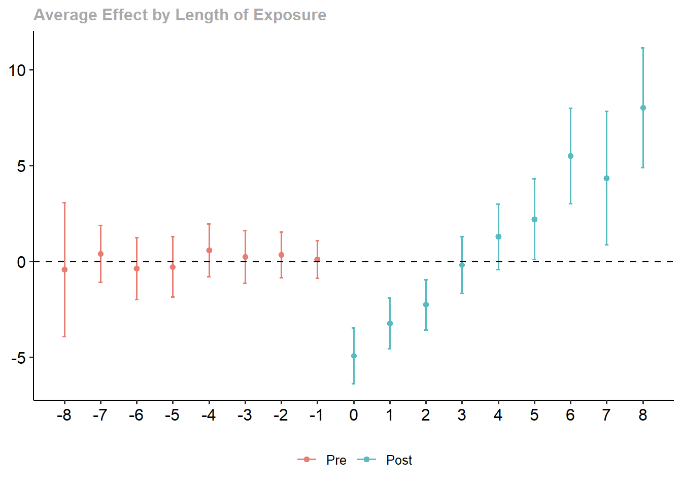

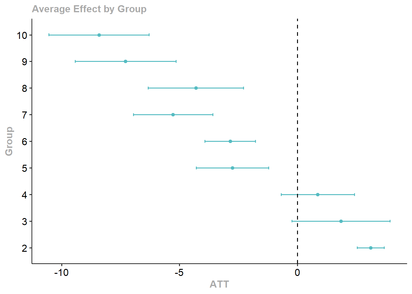
agg.gs <- aggte(drdid_result, type = "group")

ggdid(agg.gs)

---

35.12.13 Difference-in-Differences with Continuous Treatment

Most of the DiD machinery developed in this chapter, from the simple 2x2 design to the group-time estimator, has been built for a binary treatment: a unit is either treated at some time or it is not. A large slice of empirical work does not fit that template. A county may be exposed to a tariff shock whose magnitude varies across local industries (Acemoglu et al. 2016). A state may raise its minimum wage by different amounts in different years (Cengiz et al. 2019). In each of these settings the analyst observes both whether a unit was treated and how much treatment it received. The natural object of interest is no longer a single number but a function: how the average causal effect varies with the dose.

This section develops the identification and estimation of such dose-response effects in panel data. The treatment is now a continuous (or many-valued) variable \(D_i \in \mathcal{D} \subset \mathbb{R}_{\geq 0}\), where \(D_i = 0\) corresponds to no treatment and \(D_i > 0\) corresponds to varying intensities of exposure. The framework draws on De Chaisemartin and d’Haultfoeuille (2020) and De Chaisemartin and D’haultfœuille (2023) for the critique of TWFE in heterogeneous-effect settings (the published methodological backbone of the continuous case), and on Callaway et al. (2024) for the event-study extension. The story is, in spirit, the same one told in Section 35.13: naive linear specifications can quietly average over heterogeneity in ways that are difficult to defend, and the cure is to be explicit about the estimand and to estimate it directly.

---

35.12.13.1 Setup and Notation

We observe a panel of units \(i = 1, \dots, N\) over time periods \(t = 1, \dots, T\). Let \(G_i \in \{q, \dots, T, \infty\}\) denote the period in which unit \(i\) first receives a positive dose, with \(G_i = \infty\) for the never-treated. For each treated unit, \(D_i \in \mathcal{D}\) denotes the dose received from period \(G_i\) onward; the dose is assumed time-invariant within a unit for the simplest case and time-varying \(D_{it}\) in the general case. Most of the conceptual content survives in the simpler time-invariant-dose setting, so we present that first and indicate at each step how the argument generalizes.

The potential-outcomes framework extends naturally. Let \(Y_{it}(d)\) denote the outcome unit \(i\) would realize at time \(t\) under dose \(d\). The observed outcome is

\[ Y_{it} = Y_{it}(D_i) \cdot \mathbf{1}\{t \geq G_i\} + Y_{it}(0) \cdot \mathbf{1}\{t < G_i\}. \]

The novelty relative to the binary case is that we now have a continuum of counterfactuals \(\{Y_{it}(d): d \in \mathcal{D}\}\) for each unit, not just two. Identification will have to do enough work to recover an entire curve, not just a single difference.

---

35.12.13.2 Estimands

Three estimands cover almost everything the literature reports. They differ in whether they describe levels or slopes of the dose-response, and in whether they are conditioned on the treated.

The first is the dose-specific average treatment effect on the treated:

\[ ATT(d, t) = \mathbb{E}[Y_{it}(d) - Y_{it}(0) \mid D_i = d, G_i \leq t]. \]

This is the level effect of dose \(d\), evaluated at the population of units that actually received dose \(d\). As \(d\) varies, \(ATT(d, t)\) traces out a curve: the dose-response function on the treated. Reporting this curve, rather than a single scalar, is the natural deliverable of a continuous-treatment DiD analysis.

The second is the average causal response (ACR), the slope of the dose-response evaluated at dose \(d\):

\[ ACR(d, t) = \frac{\partial}{\partial d} \mathbb{E}[Y_{it}(d) - Y_{it}(0)]. \]

In words, \(ACR(d, t)\) answers: at dose level \(d\), what is the marginal effect of an additional unit of treatment, averaged over the entire population? The integral of \(ACR(\cdot, t)\) over \(\mathcal{D}\) recovers an aggregate effect.

The third is the average causal response on the treated (ACRT), the same marginal effect but conditioned on the treated population:

\[ ACRT(d, t) = \frac{\partial}{\partial d} \mathbb{E}[Y_{it}(d) - Y_{it}(0) \mid D_i = d]. \]

It is worth slowing down on this object because it is the workhorse estimand of the continuous-DiD literature and because reading the formula too quickly hides what it is actually doing. ACRT is a derivative, not a difference. It does not compare units that received dose \(d\) to units that received dose \(d'\); that would be a finite difference and would confound selection (who is at each dose) with response (how each dose affects the outcome). Instead, ACRT asks: if we held the dose-receiving population fixed at the units that actually took dose \(d\), and we shifted their dose marginally, how would their average outcome change? It is the slope of the dose-response curve at dose \(d\), evaluated for units whose dose happens to be \(d\).

The distinction between ACR and ACRT is the distinction between two questions:

• ACR(d): if a randomly selected unit from the population were given dose \(d\) rather than dose \(d - \mathrm{d}d\), how would its outcome change?
• ACRT(d): if a unit that actually took dose \(d\) were given dose \(d\) rather than dose \(d - \mathrm{d}d\), how would its outcome change?

The difference matters whenever the units that select into high doses respond differently to those doses than units that select into low doses would have. This is the selection-on-gains pattern: firms that adopt a new technology more aggressively are often the firms with the most to gain from it. ACRT averages the marginal effects over the realized treated population at each dose; ACR averages over the full population, treated or not. These objects are different functions of the same underlying dose-response surface, and choosing between them is a substantive decision about whose marginal effect the analyst wants to report.

---

35.12.13.3 Identifying Assumptions

Two assumptions do the work in the continuous-treatment DiD framework. Both have direct analogues in the binary case but require care because the counterfactual is now indexed by a continuum.

The first is no anticipation, identical in spirit to the binary-treatment version:

\[ \mathbb{E}[Y_{it}(0)] = \mathbb{E}[Y_{it} \mid G_i = g], \quad \text{for all } t < g. \]

Units do not adjust their outcomes in response to a treatment they have not yet received. This is the standard requirement and can be diagnosed with pre-treatment event-study plots in exactly the same way as in the staggered binary case.

The second is parallel trends, and here the continuous setting forces a choice. The choice has nothing to do with statistical convenience: the two versions identify different estimands, and the gap between them is precisely the selection-on-gains bias.

Weak parallel trends posits that the expected change in the never-treated potential outcome is the same for the never-treated group and for the cohort that received dose \(d\):

\[ \mathbb{E}[Y_{it}(0) - Y_{i,g-1}(0) \mid G_i = g, D_i = d] = \mathbb{E}[Y_{it}(0) - Y_{i,g-1}(0) \mid G_i = \infty], \quad \forall t \geq g, d \in \mathcal{D}. \]

This is the natural lift of the binary parallel-trends assumption: it says that, in the absence of treatment, the units that took dose \(d\) would have evolved on average like the never-treated, conditional on the cohort and dose. The assumption is just about the baseline path, not about how units would respond to alternative doses. Under weak parallel trends, \(ATT(d, t)\) and \(ACRT(d, t)\) are identified.

Here is the point worth pausing on: weak parallel trends does not assume away selection bias on the responses. Two units might satisfy weak parallel trends (they would have had the same untreated path) and still respond very differently to the same dose if their unobserved heterogeneity made them more or less responsive to that particular intensity. Under weak parallel trends, the analyst is identifying ACRT, not ACR, precisely because the selection-on-gains pattern remains inside the estimand. The ACRT curve is a curve over the realized treated population at each dose; it is informative, but it is not the population dose-response.

Strong parallel trends posits something stricter: the expected change in the dose-\(d\) potential outcome is the same across all dose subpopulations.

\[ \mathbb{E}[Y_{it}(d) - Y_{i,g-1}(d) \mid G_i = g, D_i = d'] = \mathbb{E}[Y_{it}(d) - Y_{i,g-1}(d) \mid G_i = g], \quad \forall d, d' \in \mathcal{D}. \]

In words, units that actually took dose \(d'\) would have responded the same way to dose \(d\) as units that actually took dose \(d\). Strong parallel trends is exactly the assumption that the selection-on-gains channel is shut off: there is no systematic relationship between which dose a unit took and how it would respond to a counterfactual dose. Under strong parallel trends, the population dose-response function \(ACR(d, t)\) is identified, and it coincides with the on-the-treated version \(ACRT(d, t)\).

The phrasing matters. Strong parallel trends is not a separate piece of evidence that the analyst gathers to push from ACRT to ACR; it is the explicit assumption that lets the analyst report ACR rather than ACRT. The analyst pays for the richer estimand by ruling out, by assumption, the selection-on-gains story that motivated reaching for the continuous-treatment framework in the first place. Whether that price is worth paying is a substantive question, not a technical one.

The practical default is conservative: assume the weak version, identify \(ACRT\), and report the analysis as a conditional-on-treated dose-response. The stronger version is appropriate only when there is substantive reason to believe that dose assignment is unrelated to the gains, for instance when the dose is determined by a quasi-experimental shock that varies for reasons orthogonal to the potential outcomes. A useful diagnostic, when both estimators can be computed, is to report the ACR and ACRT curves side by side; a large gap is evidence that the selection-on-gains channel is empirically active, and the population-level interpretation of ACR is on weaker footing.

---

35.12.13.4 Why TWFE Goes Wrong with Continuous Treatment

It is tempting to estimate continuous-treatment DiD by simply replacing the binary treatment indicator with the continuous dose in a TWFE regression:

\[ Y_{it} = \alpha_i + \gamma_t + \beta \cdot D_{it} + \epsilon_{it}. \]

The coefficient \(\beta\) is then interpreted as “the marginal effect of one more unit of dose.” This interpretation is correct only under restrictive conditions; in general, \(\beta\) is a weighted average of unit-time-specific marginal effects with weights that can be negative and that need not concentrate where the analyst’s substantive interest lies.

De Chaisemartin and d’Haultfoeuille (2020) make the point cleanly for binary staggered designs and the logic carries over to the continuous case. In a two-period setting with strong parallel trends and constant treatment effects across doses, the TWFE coefficient on \(D\) does recover the common marginal effect. Once treatment effects are allowed to vary with the dose (the substantively interesting case, the whole reason to do a continuous-treatment analysis in the first place), the TWFE coefficient becomes a weighted average of \(ACR(d, t)\) across doses and time periods. The weights are functions of the variance of \(D_{it}\) within unit-time cells, not of any substantive feature of the dose distribution. In the staggered-adoption case, the same negative-weight pathology that De Chaisemartin and d’Haultfoeuille (2020) diagnose for binary treatments reappears, only now compounded by the dose dimension: comparisons of high-dose-late-treated units to low-dose-early-treated units can enter the estimand with negative weight.

The practical implication is the same as in the binary case. TWFE with a continuous treatment is best treated as a descriptive summary, useful for first-look exploration and benchmark comparisons. It should not be reported as the headline estimate without an accompanying decomposition or an alternative estimator that targets a well-defined dose-response object.

---

35.12.13.5 Multi-Valued (Discrete Dose Bins) DiD

Many applications sit between the clean binary and the fully continuous cases. The dose is naturally discretized into a handful of levels: a tax rate that takes a few statutory values, a training program that comes in two-week and four-week and six-week versions, a tariff that is set in coarse brackets. The continuous-treatment estimators of the previous sections are overkill in this setting, since there is no dose continuum to smooth over, and the binary estimators throw away the dose information entirely.

The right tool is a multi-valued (discrete-dose) DiD, in which each dose level acts as a separate treatment group and the analyst recovers a vector of dose-specific ATTs. De Chaisemartin and D’haultfœuille (2023) develop the framework in detail and show that, under a weak parallel-trends assumption for each dose level, the dose-specific ATTs are identified by group-time-style estimators applied separately to each dose stratum. The aggregate object is then a small table or step-function curve rather than a smooth dose-response.

Concretely, suppose the dose takes \(K\) discrete values \(d_1 < d_2 < \dots < d_K\) in the treated population (with \(d_0 = 0\) for the never-treated). The estimand of interest is the vector

\[ \big( ATT(d_1, t), ATT(d_2, t), \dots, ATT(d_K, t) \big), \]

where each \(ATT(d_k, t)\) is identified by a DiD between units in dose group \(k\) and the never-treated, under the corresponding weak parallel-trends assumption restricted to dose group \(k\). The analyst can read the table directly or compute discrete differences \(ATT(d_{k+1}, t) - ATT(d_k, t)\) to approximate the slope of the dose-response, which is the discrete-dose analogue of ACR.

The framework subsumes two limiting cases. When \(K = 1\) (only one dose level), it reduces to the standard binary DiD. When \(K\) is large and the dose grid is fine, it approaches the continuous-treatment case from below, and the analyst should ask whether the gain in dose resolution is worth the loss of statistical power per dose stratum. The empirical sweet spot is typically \(K \in \{2, 3, 4, 5\}\): enough levels to detect non-monotonicity in the dose-response, few enough that each stratum has a usable sample size.

The estimator can be implemented in any package that supports group-time ATTs (for example, the did package by passing the dose group as the gname argument), or by hand as a stratified DiD. We illustrate both below.

---

35.12.13.6 Estimation: Demonstration First, Production Second

We work through the estimation in two passes. The first pass is a from-scratch demonstration that estimates a discrete-dose ATT vector using only base R and fixest, to make the mechanics visible. The second pass calls the canonical published-package implementations (did for the multi-valued case, the contdid CRAN package for the continuous case) on the same synthetic data.

35.12.13.6.1 Demonstration: stratified DiD by dose bin

We simulate a panel with a never-treated group and three discrete dose levels, and we recover the dose-specific ATT vector by a sequence of binary 2x2 DiDs against the never-treated.

suppressPackageStartupMessages({
  library(dplyr)
  library(tidyr)
  library(ggplot2)
  library(fixest)
})

set.seed(20240515)

# Panel: 4 dose groups (0 = never-treated, 1/2/3 = three discrete dose levels)
# 2 periods (pre and post), 1000 units per group.
n_per_group <- 1000
groups      <- 0:3
true_att    <- c(0.0, 0.5, 1.2, 1.5)  # concave dose-response on the treated

panel <- expand.grid(
  unit  = seq_len(n_per_group * length(groups)),
  time  = c(0, 1)
) %>%
  arrange(unit, time) %>%
  mutate(
    dose_group = rep(rep(groups, each = n_per_group), each = 2),
    unit_fe    = rep(rnorm(n_per_group * length(groups), sd = 0.3), each = 2),
    time_fe    = ifelse(time == 0, 0, 0.2),
    treat_post = as.integer(dose_group > 0 & time == 1),
    att_realized = true_att[dose_group + 1] * treat_post,
    Y          = unit_fe + time_fe + att_realized + rnorm(n(), sd = 0.5)
  )

head(panel)
#>   unit time dose_group     unit_fe time_fe treat_post att_realized           Y
#> 1    1    0          0  0.17321300     0.0          0            0 -0.19606350
#> 2    1    1          0  0.17321300     0.2          0            0  0.52355291
#> 3    2    0          0  0.16370894     0.0          0            0  0.21227118
#> 4    2    1          0  0.16370894     0.2          0            0 -0.09471705
#> 5    3    0          0 -0.01175345     0.0          0            0 -0.09942626
#> 6    3    1          0 -0.01175345     0.2          0            0 -0.46802315

The data are organized so the dose-response is concave: dose level 2 has a marginal effect of \(1.2 - 0.5 = 0.7\) above dose 1, while dose level 3 has a marginal effect of only \(1.5 - 1.2 = 0.3\) above dose 2. The discrete ACR is decreasing in the dose, a classic diminishing-returns pattern.

Now estimate the dose-specific ATT vector by running one 2x2 DiD per dose level against the never-treated:

att_by_dose <- lapply(setdiff(groups, 0), function(k) {
  sub <- panel %>%
    filter(dose_group %in% c(0, k)) %>%
    mutate(
      treated = as.integer(dose_group == k),
      post    = as.integer(time == 1),
      did     = treated * post
    )
  fit <- feols(Y ~ did | unit + time, data = sub)
  est <- unname(coef(fit)["did"])
  se  <- unname(sqrt(diag(vcov(fit)))["did"])
  data.frame(
    dose     = k,
    att_hat  = est,
    se       = se,
    ci_lo    = est - 1.96 * se,
    ci_hi    = est + 1.96 * se,
    att_true = true_att[k + 1]
  )
}) %>% bind_rows()

att_by_dose
#>   dose   att_hat         se     ci_lo     ci_hi att_true
#> 1    1 0.5231768 0.03282171 0.4588462 0.5875073      0.5
#> 2    2 1.2216259 0.03213804 1.1586354 1.2846165      1.2
#> 3    3 1.5451271 0.03227033 1.4818773 1.6083770      1.5

The table reports, for each discrete dose, the estimated ATT, its standard error, a 95% confidence interval, and the true ATT used to simulate the data. Compare the att_hat column to att_true: the stratified DiD recovers the dose-specific level effects without bias because each comparison is a clean 2x2 against the never-treated under satisfied parallel trends. The discrete ACR is the first difference of the att_hat column moving from one dose to the next.

Plotting the dose-response gives the headline figure:

ggplot(att_by_dose, aes(x = dose, y = att_hat)) +
  geom_pointrange(aes(ymin = ci_lo, ymax = ci_hi)) +
  geom_line(aes(y = att_true), linetype = "dashed", color = "red") +
  scale_x_continuous(breaks = 1:3) +
  labs(x = "Dose level (k)",
       y = "ATT(d_k): estimated level effect",
       title = "Dose-response from stratified DiD",
       subtitle = "Points + 95% CIs; dashed red line is the true ATT") +
  theme_minimal()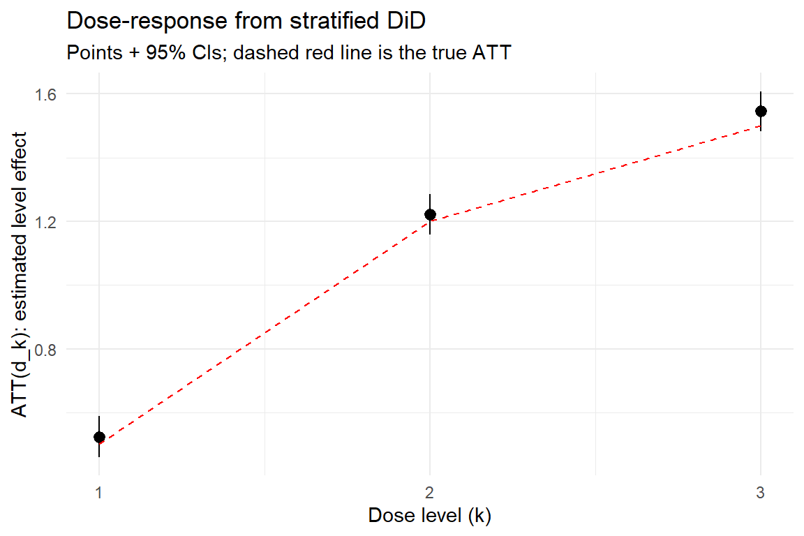

Figure 35.23: Discrete-dose ATT estimates from stratified 2x2 DiDs against the never-treated. Points are estimates, vertical lines are 95% CIs, dashed line is the true dose-response used in the simulation. The recovered curve is concave in the dose, mirroring the simulated diminishing-returns pattern.

Figure 35.23 makes the substantive story immediate: most of the gain from the program is realized at dose level 2, and the marginal benefit from moving to dose level 3 is much smaller. A reviewer who looked at a single TWFE coefficient on a continuous version of the dose would have averaged this concave pattern into a single slope and missed the diminishing-returns story.

The same logic generalizes to staggered adoption with discrete doses by replacing the single 2x2 with a group-time ATT estimator (Callaway and Sant’Anna 2021), computed separately for each dose group. We turn to the production-package implementation next.

35.12.13.6.2 Production: did for multi-valued discrete-dose DiD

The published did package by Callaway and Sant’Anna (2021) handles staggered adoption with binary treatment and extends to the discrete-multi-valued case by treating each dose group as its own cohort. The aggregation step then reports either dose-specific ATTs or a pooled effect.

# install.packages("did")  # CRAN, Callaway and Sant'Anna
library(did)

# Cast the dose group as the cohort variable. The package expects an
# integer "G" indicating period of first treatment; we encode the dose
# group by interacting it with the actual first-treatment period.
panel_did <- panel %>%
  group_by(unit) %>%
  mutate(first_treat = ifelse(dose_group == 0, 0,
                              min(time[treat_post == 1], default = 0))) %>%
  ungroup()

att_did <- att_gt(
  yname  = "Y",
  tname  = "time",
  idname = "unit",
  gname  = "first_treat",
  data   = panel_did,
  control_group = "nevertreated",
  est_method    = "dr"  # doubly robust estimator
)
summary(att_did)
ggdid(att_did)

The summary() output is a table with one row per (cohort, time-period) pair, reporting the estimated \(ATT(g, t)\), its standard error, and a 95% confidence interval. With three dose groups and two time periods, you get three estimates: one ATT per dose level at the post-period. The ggdid() figure renders each cohort’s path in its own panel; for the discrete-dose application the cohorts are the dose groups, so the panels read off the dose-response directly.

35.12.13.6.3 Production: contdid for the continuous case

When the dose is genuinely continuous (or has too many discrete levels to stratify), the contdid CRAN package by Callaway, Goodman-Bacon, and Sant’Anna implements the B-spline nonparametric estimator that targets either \(ATT(d, t)\) or \(ACRT(d, t)\) directly. The methodological paper backing the implementation is still circulating as a working paper; the published Callaway et al. (2024) covers the event-study extension and is the journal-cited reference for that part of the framework.

# install.packages("contdid")  # CRAN, Callaway, Goodman-Bacon, Sant'Anna
library(contdid)

# Generate the package's built-in simulated panel.
df_cont <- simulate_contdid_data(
  n = 5000,
  num_time_periods = 4,
  num_groups       = 4
)

# Estimate ATT(d), the level effect curve, with a uniform CB.
att_d <- cont_did(
  yname            = "Y",
  tname            = "time_period",
  idname           = "id",
  dname            = "D",
  gname            = "G",
  data             = df_cont,
  target_parameter = "level",
  aggregation      = "dose",
  treatment_type   = "continuous",
  control_group    = "notyettreated",
  biters           = 1000,
  cband            = TRUE
)
summary(att_d)
ggcont_did(att_d) +
  labs(x = "Dose D", y = "ATT(d)",
       title = "Level dose-response from contdid",
       subtitle = "Uniform 95% CB via multiplier bootstrap")

The summary(att_d) output reports the estimated \(ATT(d)\) on a fine grid of dose values, the uniform-band lower and upper limits at each grid point, and an overall test of the joint null that \(ATT(d) = 0\) for all \(d\). The ggcont_did() figure plots the curve with the uniform band shaded; the right way to read it is to scan for the dose range over which the band excludes zero (the doses for which the level effect is statistically distinguishable from zero) and to read the shape (monotone increasing, concave, threshold) rather than any single point estimate.

To recover the ACRT slope curve, change target_parameter = "slope". To trace the dynamic path, change aggregation = "eventstudy". Both are one-argument changes:

acrt_d <- cont_did(
  yname = "Y", tname = "time_period", idname = "id",
  dname = "D", gname = "G", data = df_cont,
  target_parameter = "slope",     # ACRT(d) instead of ATT(d)
  aggregation      = "dose",
  treatment_type   = "continuous",
  control_group    = "notyettreated",
  biters = 1000, cband = TRUE
)
summary(acrt_d)
ggcont_did(acrt_d) +
  labs(x = "Dose D", y = "ACRT(d)",
       title = "Marginal-effect dose-response from contdid")

The summary(acrt_d) table mirrors the level-effect table but reports the derivative of the dose-response (the marginal effect of one more unit of dose) at each grid point. A positive but declining ACRT curve is the signature of a concave dose-response; a curve that crosses zero is the signature of a non-monotone response. Comparing the level and slope figures together is the standard reporting style for a continuous-DiD analysis.

---

35.12.13.7 Diagnostics and Sensitivity

Three routine checks should accompany any continuous-DiD estimate, in addition to the pre-trend tests carried over from the binary case.

The first is a dose common-support diagnostic. Plot the empirical density of the dose among the treated and check that the range over which \(ATT(d, t)\) is estimated is well populated. The B-spline smoother will happily extrapolate into thin regions, but the resulting estimates have little to do with the data. The diagnostic plot is one line of ggplot:

panel %>%
  filter(dose_group > 0) %>%
  mutate(dose_value = dose_group) %>%
  ggplot(aes(x = dose_value)) +
  geom_bar(width = 0.4, fill = "grey70") +
  labs(x = "Dose level among treated", y = "Count",
       title = "Common-support diagnostic for the dose distribution") +
  theme_minimal()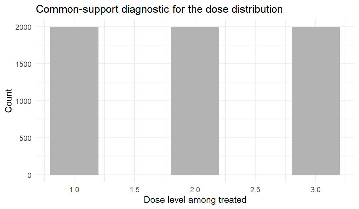

Figure 35.24: Common-support diagnostic. Density of the dose among the treated, with a rug of individual observations. The dose-response is identified only over the range where the density is non-negligible; estimates outside that range are smoother-driven extrapolation, not data.

In the discrete-dose simulation above (Figure 35.24) the support is balanced by construction (1000 units per dose level), so the diagnostic is trivially satisfied; in a real application the histogram or density would typically be far from uniform and the analyst should restrict the reported dose-response curve to doses that are well represented in the data.

The second is a placebo dose specification. Re-run the estimation, but pretend treatment occurred one period earlier than it actually did. A non-zero estimated dose-response in the placebo is evidence of pre-trends that vary with dose, which directly violates the parallel-trends assumption in its continuous-treatment form. The placebo is sharper than the standard scalar pre-trend test because it reveals whether the violation of parallel trends is itself dose-dependent.

The third is a weak-vs-strong PT comparison. Estimate the dose-response under both the weak-parallel-trends assumption (which identifies ACRT) and the strong-parallel-trends assumption (which identifies ACR). A small gap between the two curves is consistent with negligible selection-on-gains; a large gap is direct empirical evidence that the population-level interpretation of ACR rests on an assumption that the data are not willing to make. Reporting both curves, with a clear statement of which one the headline result corresponds to, is the conservative default.

---

35.12.13.8 Empirical Applications

Two published applications illustrate the design pattern in different domains.

Acemoglu et al. (2016) study the employment consequences of the rise in Chinese import competition in the United States in the 2000s. The treatment is a continuous measure of local-labor-market exposure to Chinese imports, constructed from pre-period industry shares interacted with national import-penetration changes. The dose varies smoothly across commuting zones, and the natural deliverable is the dose-response of local employment to a one-unit increase in exposure. The original paper uses a Bartik-style shift-share instrumental-variables specification layered on a long-difference design; the same data could be re-analyzed in the continuous-DiD framework to recover a non-parametric dose-response curve and check that the structural-IV linear specification is consistent with what a flexible estimator finds.

Cengiz et al. (2019) estimate the effect of minimum-wage increases on the number of low-wage jobs. The treatment is a continuous wage floor that varies across states and years, with substantial heterogeneity in the size of the bite. The analysis is structured as a bunching design (counting jobs disappearing from below the new floor and reappearing above it), which is conceptually adjacent to a dose-response but reports a different estimand. A continuous-DiD analysis on the same panel would directly trace out how employment effects scale with the magnitude of the minimum-wage change, with the dose interpreted either as the level of the new minimum wage or as the size of the increase relative to the prevailing market wage.

A third application shows most directly what a flexible dose-response buys over a linear specification. Acemoglu and Finkelstein (2008) study a 1983 Medicare reform that eliminated a labor subsidy for hospitals, changing the relative price of capital and labor by an amount that varied across hospitals according to their pre-reform input mix. The dose is the size of that price change, and the outcome is the capital-labor ratio. A two-way fixed-effects regression reports a significant increase in capital intensity. A nonparametric continuous-DiD re-analysis recovers an effect on the order of an eighteen percent increase, roughly half again as large as the TWFE estimate, a gap that reflects the weighting that TWFE imposes under heterogeneous responses. More revealing than the headline magnitude is the shape: the estimated average causal response is large and positive at low subsidy levels and flattens, even turning slightly negative, at higher doses. That pattern sits uneasily with a simple two-factor production model and with the strong-parallel-trends assumption needed to compare nonzero doses, so the qualitative conclusion that hospitals shifted toward capital survives while any precise reading of which subsidy levels matter most does not. The lesson generalizes: a linear dose specification can deliver the right sign and a misleading magnitude and an entirely hidden shape.

In all three cases the substantive payoff of the continuous framework is the ability to detect non-linearities in the dose-response that a binary specification would average away: a tariff exposure that bites hardest in the middle of its range, a minimum-wage increase whose employment cost rises faster than linearly past a threshold, an input subsidy whose effect is concentrated at the low end of its range.

---

35.12.13.9 When to Use Continuous-Treatment DiD

The continuous-treatment DiD framework is the right tool when the substantive question concerns the shape of a dose-response, not merely the average effect of being treated. It is also the right tool when dose heterogeneity is large enough that an average-of-treated-effects estimate would conflate compositional and behavioral channels. The price of moving to the dose-response framework is paid in three places: data requirements (one needs enough variation in the dose to identify the curve), assumption strength (one must choose between the weak and strong forms of parallel trends and live with the implications of each), and inference complexity (uniform confidence bands and bootstrap iterations replace the simple standard errors of the binary case).

When the dose is naturally discrete with a small number of levels, the multi-valued DiD framework is a strict improvement over both the binary and the smooth-continuous alternatives: it preserves the dose information, makes the dose-specific ATTs visible, and avoids the implicit smoothing assumptions that a continuous estimator imposes. When the dose is genuinely continuous, the continuous-treatment estimators are the right choice, but the analyst should report the diagnostic comparison with a discretized version of the same data as a robustness check on the smoothing assumptions.

Several alternative designs cover related but distinct questions. The shift-share / Bartik design handles continuous local-labor-market exposure under a structural identification argument that is complementary to the parallel-trends argument used here; in many applications both are reported as robustness checks on each other. The generalized synthetic control and matrix completion estimator target the same panel structure but with a factor-model identification strategy that does not require a dose-response framing. The matching-based GPS dose-response analysis in the matching chapter handles cross-sectional dose-response without a panel, at the cost of a stronger conditional-unconfoundedness assumption. The choice among these designs is the same kind of choice the analyst faces in the binary case: which set of assumptions is least uncomfortable in this dataset, and which estimand is closest to the substantive question.

35.12.14 Nonlinear Difference-in-Differences

Notation in this section follows the conventions of Table 31.12 in the foundations chapter.

The standard Difference-in-Differences estimator assumes that the untreated potential outcome trends linearly across groups: in the absence of treatment, the treated and control groups would have moved on parallel lines. This is a defensible assumption for continuous outcomes that range freely over the real line (log earnings, log expenditure, voter share), but it breaks down when the outcome is bounded, discrete, or otherwise constrained. A linear trend that produces an “untreated employment rate” of \(-0.05\) or a “predicted churn proportion” of \(1.13\) has not actually predicted anything, and an estimator built on top of such a prediction is mis-specified in a way the linear specification will not flag.

The cases where this matters are common in applied work:

• Binary outcomes, such as employment status, default indicators, or whether a customer renewed a contract. The outcome is bounded in \(\{0, 1\}\) and the conditional mean lies in \([0, 1]\).
• Fractional outcomes, such as the proportion of a firm’s customers who churned, the share of a portfolio invested in a particular asset, or the fraction of households in poverty. The outcome lies in \([0, 1]\).
• Count outcomes, such as the number of crimes in a neighborhood, the number of patents filed by a firm, or the number of insurance claims per policyholder. The outcome is a non-negative integer with a discrete distribution.

For each of these, the natural model of the conditional mean is nonlinear: a logistic or probit link for binary and fractional outcomes, an exponential link for counts. Linear parallel trends imposed on such outcomes can produce qualitatively wrong inferences, including effects with the wrong sign in regions of the covariate space where the linear approximation is at its worst. The framework developed below, drawing on Wooldridge (2023), replaces linear parallel trends with a parallel trends in a transformed index, which respects the constrained nature of the outcome while preserving the DiD logic of canceling unit and time fixed effects through differencing.

The remainder of this section develops the framework in three parts: an overview of the nonlinear conditional-mean structure, the identifying assumptions (a conditional no-anticipation condition and a conditional index-parallel-trends condition), and two equivalent estimators (an imputation estimator and a pooled QMLE).

---

35.12.14.1 Overview of Framework

We consider a panel dataset where units are observed over \(T\) time periods. Units become treated at various times (staggered rollout), and the goal is to estimate Average Treatment Effect on the Treated (ATT) at different times.

Let \(Y_{it}(g)\) denote the potential outcome at time \(t\) if unit \(i\) were first treated in period \(g\), where \(g = q, \ldots, T\) for treated cohorts. Let \(Y_{it}(0)\) denote the never-treated potential outcome. Define the ATT for cohort \(g\) at time \(r \geq g\) as:

\[ \tau_{gr} = \mathbb{E}\left[Y_{ir}(g) - Y_{ir}(0) \mid D_g = 1\right] \]

Here, \(D_g = 1\) indicates that unit \(i\) was first treated in period \(g\).

Rather than assuming linear conditional expectations of untreated outcomes, we posit a nonlinear conditional mean using a known, strictly increasing function \(G(\cdot)\):

\[ \mathbb{E}[Y_{it}(0) \mid D, X] = G\left( \alpha + \sum_{g=q}^{T} \beta_g D_g + X \kappa + \sum_{g=q}^{T} (D_g \cdot X)\eta_g + \gamma_t + X \pi_t \right) \]

This formulation nests logistic and Poisson mean structures, and allows us to handle various limited dependent variables.

---

35.12.14.2 Assumptions

Identification of the nonlinear DiD ATT requires two assumptions, each a natural extension of the standard linear DiD assumptions to the nonlinear setting.

The first is Conditional No Anticipation: prior to treatment, the conditional mean of the eventually-treated cohort does not differ systematically from the conditional mean it would have had under permanent non-treatment. Formally,

\[ \mathbb{E}[Y_{it}(g) \mid D_g = 1, X] = \mathbb{E}[Y_{it}(0) \mid D_g = 1, X], \quad \forall t < g. \]

In words, the cohort treated at \(g\) does not adjust its behavior in anticipation of treatment in the periods before \(g\). This is the same assumption as in linear DiD; the only difference is that it is now phrased in terms of the conditional mean of the transformed outcome rather than the level. Anticipation, where present, manifests as a divergence of the cohort’s pre-treatment conditional means from the untreated counterfactual, and it can be diagnosed in the same way as in standard event-study plots.

The second is Conditional Index Parallel Trends: the untreated mean trends are parallel after passing through a known monotone transformation \(G(\cdot)\). Formally,

\[ \mathbb{E}[Y_{it}(0) \mid D, X] = G(\text{linear index in } D, X, t), \]

where \(G\) is strictly increasing and known up to its functional form (e.g., \(G(\cdot) = \exp(\cdot)\) for Poisson outcomes, or the logistic CDF \(G(\cdot) = \Lambda(\cdot)\) for binary outcomes). The choice of \(G\) is dictated by the outcome: count outcomes call for the exponential, binary outcomes for the logistic or probit, and so on. The substantive content of the assumption is that on the index scale (the argument of \(G\)), trends are parallel across groups; on the outcome scale they are parallel only after the transformation, which is what allows the model to respect the bounds on the outcome.

These assumptions are weaker than linear parallel trends in two ways. First, they accommodate bounded outcomes without imposing implausible counterfactuals. Second, they allow for cross-group differences in the transformation that the linear specification would force into the residual. The trade-off is that the analyst must commit to a specific link function \(G\), and a mis-specified link can re-introduce some of the bias that the framework was meant to remove.

---

35.12.14.3 Estimation

Step 1: Imputation Estimator

1. Estimate Parameters Using Untreated Observations Only:

Use all \((i,t)\) such that unit \(i\) is untreated at \(t\) (i.e., \(W_{it} = 0\)). Fit the nonlinear regression model: \[ Y_{it} = G\left(\alpha + \sum_g \beta_g D_g + X_i \kappa + D_g X_i \eta_g + \gamma_t + X_i \pi_t\right) + \varepsilon_{it} \]

2. Impute Counterfactual Outcomes for Treated Observations:

For treated observations \((i,t)\) with \(W_{it}=1\), predict \(\widehat{Y}_{it}(0)\) using the model from Step 1.

3. Compute ATT for Each Cohort \(g\) and Time \(r\):

\[ \hat{\tau}_{gr} = \frac{1}{N_{gr}} \sum_{i: D_g=1} \left( Y_{ir} - \widehat{Y}_{ir}(0) \right) \]

---

Step 2: Pooled QMLE Estimator (Equivalent When Using Canonical Link)

1. Fit Model Using All Observations:

Fit the pooled nonlinear model across all units and time: \[ Y_{it} = G\left(\alpha + \sum_g \beta_g D_g + X_i \kappa + D_g X_i \eta_g + \gamma_t + X_i \pi_t + \delta_r \cdot W_{it} + W_{it} X_i \xi \right) + \varepsilon_{it} \]

Where:

• \(W_{it} = 1\) if unit \(i\) is treated at time \(t\)

• \(W_{it} = 0\) otherwise

2. Estimate \(\delta_r\) as the ATT for cohort \(g\) in period \(r\):

• \(\delta_r\) is interpreted as an event-time ATT
• This estimator is consistent when \(G^{-1}(\cdot)\) is the canonical link (e.g., log link for Poisson)

3. Average Partial Effect (APE) for ATT:

\[ \hat{\tau}_{gr} = \frac{1}{N_g} \sum_{i: D_g=1} \left[ G\left( X_i\beta + \delta_r + \ldots \right) - G\left( X_i\beta + \ldots \right) \right] \]

Canonical Links in Practice

Conditional Mean	LEF Density	Suitable For
\(G(z) = z\)	Normal	Any response
\(G(z) = \exp(z)\)	Poisson	Nonnegative/counts, no natural upper bound
\(G(z) = \text{logit}^{-1}(z)\)	Binomial	Nonnegative, known upper bound
\(G(z) = \text{logit}^{-1}(z)\)	Bernoulli	Binary or fractional responses

---

35.12.14.4 Inference

• Standard errors can be obtained via the delta method or bootstrap
• Cluster-robust standard errors by unit are preferred
• When using QMLE, the estimates are valid under correct mean specification, regardless of higher moments

When Do Imputation and Pooled Methods Match?

• They are numerically identical when:
  • Estimating with the canonical link function
  • Model is correctly specified
  • Same data used for both (i.e., W_it = 0 and pooled)

---

35.12.14.5 Application Using etwfe

The etwfe package provides a unified, user-friendly interface for estimating staggered treatment effects using generalized linear models. It is particularly well-suited for nonlinear outcomes, such as binary, fractional, or count data.

We’ll now demonstrate how to apply etwfe to estimate Average Treatment Effect on the Treated (ATT) under a nonlinear DiD framework using a Poisson model. This aligns with the exponential conditional mean assumption discussed earlier.

1. Install and load packages

# --- 1) Load packages ---
# install.packages("fixest")
# install.packages("marginaleffects")
# install.packages("etwfe")
# install.packages("ggplot2")
# install.packages("modelsummary")

library(etwfe)
library(fixest)
library(marginaleffects)
library(ggplot2)
library(modelsummary)
set.seed(12345)

2. Simulate a known data-generating process

Imagine a multi-period business panel where each “unit” is a regional store or branch of a large retail chain. Half of these stores eventually receive a new marketing analytics platform at some known time, which in principle changes their performance metric (e.g., weekly log sales). The other half never receive the platform, functioning as a “never-treated” control group.

• We have \(N=200\) stores (half eventually treated, half never treated).

• Each store is observed over \(T=10\) time periods (e.g., quarters or years).

• The true “treatment effect on the treated” is constant at \(\delta = -0.05\) for all post-treatment times. (Interpretation: the new marketing platform reduced log-sales by about 5 percent, though in real life one might expect a positive effect!)

• Some stores are “staggered” in the sense that they adopt in different periods. We’ll randomly draw their adoption date from \(\{4,5,6\}\). Others never adopt at all.

• We include store-level intercepts, time intercepts, and idiosyncratic noise to make it more realistic.

# --- 2) Simulate Data ---
N <- 200   # number of stores
T <- 10    # number of time periods
id   <- rep(1:N, each = T)
time <- rep(1:T, times = N)

# Mark half of them as eventually treated, half never
treated_ids <- sample(1:N, size = N/2, replace = FALSE)
is_treated  <- id %in% treated_ids

# Among the treated, pick an adoption time 4,5, or 6 at random
adopt_time_vec <- sample(c(4,5,6), size = length(treated_ids), replace = TRUE)
adopt_time     <- rep(0, N) # 0 means "never"
adopt_time[treated_ids] <- adopt_time_vec

# Store effects, time effects, control variable, noise
alpha_i <- rnorm(N, mean = 2, sd = 0.5)[id]
gamma_t <- rnorm(T, mean = 0, sd = 0.2)[time]
xvar    <- rnorm(N*T, mean = 1, sd = 0.3)
beta    <- 0.10
noise   <- rnorm(N*T, mean = 0, sd = 0.1)

# True treatment effect = -0.05 for time >= adopt_time
true_ATT <- -0.05
D_it     <- as.numeric((adopt_time[id] != 0) & (time >= adopt_time[id]))

# Final outcome in logs:
y <- alpha_i + gamma_t + beta*xvar + true_ATT*D_it + noise

# Put it all in a data frame
simdat <- data.frame(
    id         = id,
    time       = time,
    adopt_time = adopt_time[id],
    treat      = D_it,
    xvar       = xvar,
    logY       = y
)

head(simdat)
#>   id time adopt_time treat      xvar     logY
#> 1  1    1          6     0 1.4024608 1.317343
#> 2  1    2          6     0 0.5226395 2.273805
#> 3  1    3          6     0 1.3357914 1.517705
#> 4  1    4          6     0 1.2101680 1.759481
#> 5  1    5          6     0 0.9953143 1.771928
#> 6  1    6          6     1 0.8893066 1.439206

In this business setting, logY represents the natural log of revenue, sales, or another KPI, and xvar represents a log of local population, the number of competitor stores in the region, or a comparable covariate.

3. Estimate with etwfe

We want to test whether the new marketing analytics platform has changed the log outcome. We will use etwfe:

• fml = logY ~ xvar says that logY is the outcome, xvar is a control.

• tvar = time is the time variable.

• gvar = adopt_time is the group/cohort variable (the “first treatment time” or 0 if never).

• vcov = ~id clusters standard errors at the store level.

• cgroup = "never": We specify that the never-treated units form our comparison group. This ensures we can see pre-treatment and post-treatment dynamic effects in an event-study plot.

# --- 3) Estimate with etwfe ---
mod <- etwfe(
    fml    = logY ~ xvar,
    tvar   = time,
    gvar   = adopt_time,
    data   = simdat,
    # xvar   = moderator, # Heterogenous Treatment Effects
    vcov   = ~id,
    cgroup = "never"  # so that never-treated are the baseline
)

The raw coefficient list is uninformative on its own because the model is fully saturated with interactions. The substantive output is the aggregated treatment effects, which we obtain next.

4. Recover the ATT

Here’s a single-number estimate of the overall average effect on the treated, across all times and cohorts:

# --- 4) Single-number ATT ---
ATT_est <- emfx(mod, type = "simple")
print(ATT_est)
#> 
#>  .Dtreat Estimate Std. Error     z Pr(>|z|)    S  2.5 %  97.5 %
#>     TRUE  -0.0707     0.0178 -3.97   <0.001 13.8 -0.106 -0.0358
#> 
#> Term: .Dtreat
#> Type: response
#> Comparison: TRUE - FALSE

You should see an estimate near the true \(-0.05\).

5. Recover an event-study pattern of dynamic effects

To check pre- and post-treatment dynamics, we ask for an event study via type = "event". This shows how the outcome evolves around the adoption time. Negative “event” values correspond to pre-treatment, while nonnegative “event” values are post-treatment. The output below reports the dynamic ATT estimates by relative period.

# --- 5) Event-study estimates ---
mod_es <- emfx(mod, type = "event")
mod_es
#> 
#>  event Estimate Std. Error      z Pr(>|z|)    S   2.5 %   97.5 %
#>     -5 -0.04132     0.0467 -0.885  0.37616  1.4 -0.1328  0.05019
#>     -4 -0.01120     0.0282 -0.397  0.69172  0.5 -0.0665  0.04415
#>     -3  0.01747     0.0226  0.772  0.43987  1.2 -0.0269  0.06179
#>     -2 -0.00912     0.0193 -0.472  0.63677  0.7 -0.0469  0.02872
#>     -1  0.00000         NA     NA       NA   NA      NA       NA
#>      0 -0.08223     0.0206 -3.996  < 0.001 13.9 -0.1226 -0.04189
#>      1 -0.06108     0.0209 -2.926  0.00343  8.2 -0.1020 -0.02017
#>      2 -0.07094     0.0225 -3.159  0.00158  9.3 -0.1149 -0.02693
#>      3 -0.07383     0.0189 -3.907  < 0.001 13.4 -0.1109 -0.03680
#>      4 -0.07330     0.0334 -2.197  0.02804  5.2 -0.1387 -0.00790
#>      5 -0.06527     0.0284 -2.295  0.02175  5.5 -0.1210 -0.00952
#>      6 -0.05661     0.0402 -1.407  0.15942  2.6 -0.1355  0.02225
#> 
#> Term: .Dtreat
#> Type: response
#> Comparison: TRUE - FALSE


# Renaming function to replace ".Dtreat" with something more meaningful
rename_fn = function(old_names) {
  new_names = gsub(".Dtreat", "Period post treatment =", old_names)
  setNames(new_names, old_names)
}

modelsummary(
  list(mod_es),
  shape       = term:event:statistic ~ model,
  coef_rename = rename_fn,
  gof_omit    = "Adj|Within|IC|RMSE",
  stars       = TRUE,
  title       = "Event study",
  notes       = "Std. errors are clustered at the id level"
)

Event study

	(1)
+ p < 0.1, * p < 0.05, ** p < 0.01, *** p < 0.001
Std. errors are clustered at the id level
Period post treatment = -5	-0.041
	(0.047)
Period post treatment = -4	-0.011
	(0.028)
Period post treatment = -3	0.017
	(0.023)
Period post treatment = -2	-0.009
	(0.019)
Period post treatment = -1	0.000
Period post treatment = 0	-0.082***
	(0.021)
Period post treatment = 1	-0.061**
	(0.021)
Period post treatment = 2	-0.071**
	(0.022)
Period post treatment = 3	-0.074***
	(0.019)
Period post treatment = 4	-0.073*
	(0.033)
Period post treatment = 5	-0.065*
	(0.028)
Period post treatment = 6	-0.057
	(0.040)
Num.Obs.	2000
R2	0.235
FE..adopt_time	X
FE..time	X

• By default, this will return events from (roughly) the earliest pre-treatment period up to the maximum possible post-treatment period in your data, using never-treated as the comparison group.

• Inspect the estimates and confidence intervals. Ideally, pre-treatment estimates should be near 0, and post-treatment estimates near \(-0.05\).

6. Plot the estimated event-study vs. the true effect

In a business or marketing study, a useful final step is a chart showing the point estimates (with confidence bands) plus the known true effect as a reference.

Construct the “true” dynamic effect curve

• Pre-treatment periods: effect = 0

• Post-treatment periods: effect = \(\delta=-0.05\)

Below we will:

1. Extract the estimated event effects from mod_es.

2. Build a reference dataset with the same event times.

3. Plot both on the same figure.

Figure 35.25 overlays the estimated ETWFE event-study with the known data-generating-process effect.

# --- 6) Plot results vs. known effect ---
est_df <- as.data.frame(mod_es)

range_of_event <- range(est_df$event)
event_breaks   <- seq(range_of_event[1], range_of_event[2], by = 1)
true_fun <- function(e) ifelse(e < 0, 0, -0.05)
event_grid <- seq(range_of_event[1], range_of_event[2], by = 1)
true_df <- data.frame(
    event       = event_grid,
    true_effect = sapply(event_grid, true_fun)
)

ggplot() +
    # Confidence interval ribbon (put it first so it's behind everything)
    geom_ribbon(
        data = est_df,
        aes(x = event, ymin = conf.low, ymax = conf.high),
        fill = "grey60",   # light gray fill
        alpha = 0.3
    ) +
    # Estimated effect line
    geom_line(
        data = est_df,
        aes(x = event, y = estimate),
        color = "black",
        size = 1
    ) +
    # Estimated effect points
    geom_point(
        data = est_df,
        aes(x = event, y = estimate),
        color = "black",
        size = 2
    ) +
    # Known true effect (dashed red line)
    geom_line(
        data = true_df,
        aes(x = event, y = true_effect),
        color = "red",
        linetype = "dashed",
        linewidth = 1
    ) +
    # Horizontal zero line
    geom_hline(yintercept = 0, linetype = "dotted") +
    # Vertical line at event = 0 for clarity
    geom_vline(xintercept = 0, color = "gray40", linetype = "dashed") +
    # Make sure x-axis breaks are integers
    scale_x_continuous(breaks = event_breaks) +
    labs(
        title = "Event-Study Plot vs. Known True Effect",
        subtitle = "Business simulation with new marketing platform adoption",
        x = "Event time (periods relative to adoption)",
        y = "Effect on log-outcome (ATT)",
        caption = "Dashed red line = known true effect; Shaded area = 95% CI"
    ) +
    causalverse::ama_theme()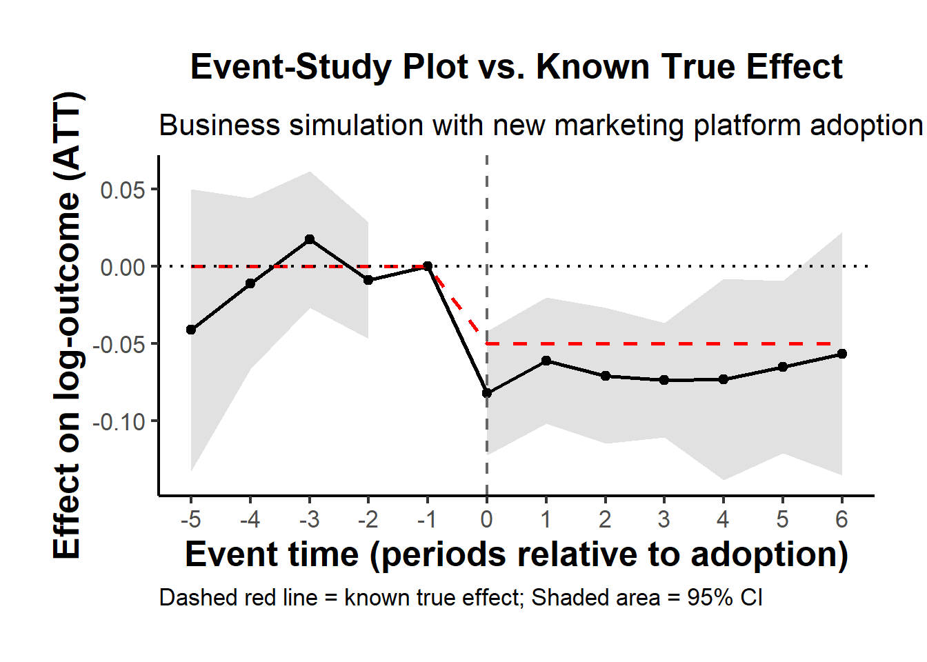

Figure 35.25: ETWFE event-study point estimates and 95% confidence band overlaid on the known true dynamic effect from the data-generating process.

• Solid line and shaded region: the ETWFE point estimates and their 95% confidence intervals, for each event time relative to adoption.

• Dashed red line: the true effect that we built into the DGP.

If the estimation works well (and your sample is big enough), the estimated event-study effects should hover near the dashed red line post-treatment, and near zero pre-treatment.

Alternatively, we could also use the plot function to produce a quick plot. Figure 35.26 shows the same event-study via the package’s built-in ribbon plot.

plot(
    mod_es,
    type = "ribbon",
    # col  = "",# color
    xlab = "",
    main = "",
    sub  = "",
    # file = "event-study.png", width = 8, height = 5. # save file
)

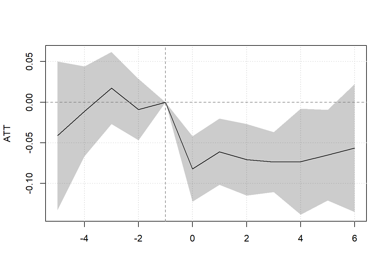
Figure 35.26: Default ribbon plot of the ETWFE event-study from marginaleffects::plot, showing the dynamic ATT estimates with their 95% confidence band.

7. Double-check in a regression table (optional)

If you like to see a clean numeric summary of the dynamic estimates by period, you can pipe your event-study object into modelsummary. The chunk below renders the resulting wide-format table.

# --- 7) Optional table for dynamic estimates ---
modelsummary(
    list("Event-Study" = mod_es),
    shape     = term + statistic ~ model + event,
    gof_map   = NA,
    coef_map  = c(".Dtreat" = "ATT"),
    title     = "ETWFE Event-Study by Relative Adoption Period",
    notes     = "Std. errors are clustered by store ID"
)

---

35.13 Modern Concerns in DiD

Roth et al. (2023) provide a comprehensive synthesis of the recent DiD literature; readers may consult that paper as a roadmap to many of the techniques discussed in this chapter, including staggered adoption, heterogeneous treatment effects, parallel-trends sensitivity analysis, and conditional/relaxed identifying assumptions.

A useful way to organize the rest of this chapter is to recognize that “what could go wrong with DiD” decomposes into a small number of recurring failure modes, and that most of the modern toolkit is a targeted response to one (or several) of them. Heterogeneous and time-varying treatment effects break the implicit weighting in two-way fixed effects, motivating the staggered-adoption estimators introduced in Section 35.12 and the Goodman-Bacon decomposition. Departures from parallel trends motivate visual diagnostics in Section 35.2, the placebo tests below, and the partial-identification machinery at the end of this chapter. Selection on observables that vary across treated and control units pulls in matching and the conditional ignorability and overlap assumptions. Functional-form sensitivity, especially with zero-valued outcomes, motivates the changes-in-changes estimator and the proportional-effects approach below. Reading the rest of the chapter as a menu indexed by failure mode (rather than as a list of unrelated diagnostics) makes it easier to know which tool is the right one to reach for, and the closing sections show how a credible DiD analysis layers several of them.

---

35.13.1 Multiple Treatments

In some settings, researchers encounter two (or more) treatments rather than a single treatment-and-control comparison. This is more than a notational nuisance: with multiple treatments operating on overlapping populations, the standard DiD machinery can collapse identification onto contrasts the analyst did not intend, and the apparent treatment effect can shift depending on which group is implicitly used as a control. Fricke (2017) provides a careful treatment of the identification challenges that arise in this setting, and the principles below distil the practical implications.

Key Principles When Dealing with Multiple Treatments

1. Always include all treatment groups in a single regression model.

   • This ensures proper identification of treatment-specific effects while maintaining a clear comparison against the control group.

2. Never use one treated group as a control for the other.

   • Running separate regressions for each treatment group can lead to biased estimates because each treatment group may differ systematically from the control group in ways that a separate model cannot fully capture.

3. Compare the significance of treatment effects (\(\delta_1\) vs. \(\delta_2\)).

   • Instead of assuming equal effects, we should formally test whether the effects of the two treatments are statistically different using an F-test or Wald test:

   \[ H_0: \delta_1 = \delta_2 \]

   • If we reject \(H_0\), we conclude that the two treatments have significantly different effects.

---

35.13.2 Multiple Treatment Groups: Model Specification

A properly specified DiD regression model with two treatments takes the following form:

\[ \begin{aligned} Y_{it} &= \alpha + \gamma_1 Treat1_{i} + \gamma_2 Treat2_{i} + \lambda Post_t \\ &+ \delta_1(Treat1_i \times Post_t) + \delta_2(Treat2_i \times Post_t) + \epsilon_{it} \end{aligned} \]

where:

• \(Y_{it}\) = Outcome variable for individual \(i\) at time \(t\).
• \(Treat1_i\) = 1 if individual \(i\) is in Treatment Group 1, 0 otherwise.
• \(Treat2_i\) = 1 if individual \(i\) is in Treatment Group 2, 0 otherwise.
• \(Post_t\) = 1 for post-treatment period, 0 otherwise.
• DiD coefficients:
  • \(\delta_1\) = Effect of Treatment 1.
  • \(\delta_2\) = Effect of Treatment 2.
• \(\epsilon_{it}\) = Error term.

---

35.13.3 Understanding the Control Group in Multiple Treatment DiD

One common concern in multiple-treatment DiD models is how to properly define the control group. A well-specified model ensures that:

• The control group consists only of untreated individuals, not individuals from another treatment group.
• The reference category in the regression represents the control group (i.e., individuals with \(Treat1_i = 0\) and \(Treat2_i = 0\)).
• If \(Treat1_i = 1\), then \(Treat2_i = 0\) and vice versa.

Failing to correctly specify the control group could lead to incorrect estimates of treatment effects. For example, omitting one of the treatment indicators could unintentionally redefine the control group as a mix of treated and untreated individuals.

---

35.13.4 Alternative Approaches: Separate Regressions vs. One Model

A common question is whether to run one large regression including all treatment groups or to run separate DiD models on subsets of the data. Each approach has implications:

1. One Model Approach (Preferred)

• Running one comprehensive regression allows for direct comparison between treatment effects in a statistically valid way.
• The interaction terms (\(\delta_1, \delta_2\)) ensure that each treatment effect is estimated relative to a common control group.
• The F-test (or Wald test) enables a formal test of whether the two treatments have significantly different effects.

2. Separate Regressions Approach

• Running separate DiD models for each treatment group can still be valid, but:
  • The estimated treatment effects are less efficient because they come from separate samples.
  • Comparisons become less straightforward, as they rely on confidence interval overlap rather than direct hypothesis testing.
  • If homoscedasticity holds (i.e., equal error variances across groups), the separate regressions approach is unnecessary. The combined model is more efficient.

Thus, unless there is strong justification for separate regressions (e.g., significant heterogeneity in error variance), the one-model approach is preferred.

---

35.13.5 Handling Treatment Intensity

In some cases, treatments differ not just in type, but also in intensity (e.g., low vs. high treatment exposure). If we observe different levels of treatment intensity, we can model it using a single categorical variable rather than multiple treatment dummies:

Rather than coding separate dummies for each treatment group, we define a multi-valued treatment variable:

\[ Y_{it} = \alpha + \sum_{j=1}^{J} \beta_j (Treatment_j \times Post_t) + \lambda Post_t + \epsilon_{it} \]

where:

• \(Treatment_j\) is a categorical variable indicating whether an individual belongs to the control group, low-intensity treatment, or high-intensity treatment.
• This approach allows for cleaner implementation and avoids excessive interaction terms.

This approach has the advantage of:

• Automatically setting the control group as the reference category.

• Ensuring correct interpretation of coefficients for different treatment levels.

35.13.6 Considerations When Individuals Can Move Between Treatment Groups

One potential complication in multiple-treatment DiD settings is when individuals can switch treatment groups over time (e.g., moving from low-intensity to high-intensity treatment after policy implementation).

• If movement is rare, it may not significantly affect estimates.

• If movement is frequent, it creates a challenge in causal identification because treatment effects might be confounded by self-selection.

A possible solution is to use an intention-to-treat (ITT) approach, where treatment assignment is based on the initially assigned group, regardless of whether individuals later switch.

35.13.7 Parallel Trends Assumption in Multiple-Treatment DiD

• Just as in standard DiD, a key assumption in multiple-treatment DiD models is that the treatment and control groups would have followed parallel trends in the absence of treatment.

• With multiple treatments, we must check pre-trends separately for each treated group against the control group.

• If pre-treatment trends are not parallel, we may need to adopt alternative methods such as synthetic control models or event study analyses.

It is worth noting how multiple-treatment settings interact with the staggered-adoption literature. Once treatments differ in timing as well as in type, the pathologies surveyed in Section 35.7 reappear: each treated arm becomes both a treated unit relative to the never-treated and a potential “forbidden comparison” for some other arm in a two-way fixed-effects regression. Reaching for the group-time average treatment effect framework, the cohort ATT estimator, or the stacked DiD design is often more defensible than trying to extend the canonical interaction model to many treatment arms by hand.

---

35.14 Mediation Under DiD

Mediation analysis helps determine whether a treatment affects the outcome directly or through an intermediate variable (mediator). In a DiD framework, this allows us to separate:

1. Direct effects: The effect of the treatment on the outcome independent of the mediator.
2. Indirect (mediated) effects: The effect of the treatment that operates through the mediator.

This is useful when a treatment consists of multiple components or when we want to understand mechanisms behind an observed effect.

---

35.14.1 Mediation Model in DiD

To incorporate mediation, we estimate two equations:

Step 1: Effect of Treatment on the Mediator

\[ M_{it} = \alpha + \gamma Treat_i + \lambda Post_t + \delta (Treat_i \times Post_t) + \epsilon_{it} \] where:

• \(M_{it}\) = Mediator variable (e.g., job search intensity, firm investment, police presence).
• \(\delta\) = Effect of the treatment on the mediator (capturing how the treatment changes \(M\)).

Step 2: Effect of Treatment and Mediator on the Outcome

\[ Y_{it} = \alpha' + \gamma' Treat_i + \lambda' Post_t + \delta' (Treat_i \times Post_t) + \theta M_{it} + \epsilon'_{it} \] where:

• \(Y_{it}\) = Outcome variable (e.g., employment, crime rate, firm performance).
• \(\theta\) = Effect of the mediator on the outcome.
• \(\delta'\) = Direct effect of the treatment (controlling for the mediator).

---

35.14.2 Interpreting the Results

• If \(\theta\) is statistically significant, it suggests that mediation is occurring (i.e., the treatment affects the outcome partly through the mediator).
• If \(\delta'\) is smaller than \(\delta\), this indicates that part of the treatment effect is explained by the mediator. The remaining portion of \(\delta'\) represents the direct effect.

Thus, we can decompose the total treatment effect as:

\[ \text{Total Effect} = \delta' + (\theta \times \delta) \]

where:

• \(\delta'\) = Direct effect (holding the mediator constant).

• \(\theta \times \delta\) = Indirect (mediated) effect.

---

35.14.3 Challenges in Mediation Analysis for DiD

Mediation in a DiD setting introduces several challenges that require careful consideration:

1. Potential Confounding of the Mediator

• A key assumption is that no unmeasured confounders affect both the mediator and the outcome.
• If such confounders exist, estimates of \(\theta\) may be biased.

2. Mediator-Outcome Endogeneity

• If the mediator is itself influenced by unobserved factors correlated with the outcome, it introduces endogeneity, making direct OLS estimates of \(\theta\) problematic.
• For example, in a crime policy evaluation:
  • The number of police officers (mediator) may be influenced by crime rates (outcome), leading to reverse causality.

3. Interaction Between Multiple Mediators

• If there are multiple mediators (e.g., a policy that increases both police presence and surveillance cameras), they may interact with each other.
• A useful test is to regress each mediator on treatment and other mediators. If a mediator predicts another, their effects are not independent, complicating interpretation.

---

35.14.4 Alternative Approach: Instrumental Variables for Mediation

One way to address mediator endogeneity is to use instrumental variables, where treatment serves as an instrument for the mediator:

Two-Stage Estimation:

1. First Stage: Predict the Mediator Using the Treatment \[ M_{it} = \alpha + \pi Treat_i + \lambda Post_t + \delta (Treat_i \times Post_t) + \nu_{it} \]
2. Second Stage: Predict the Outcome Using the Instrumented Mediator \[ Y_{it} = \alpha' + \gamma' Treat_i + \lambda' Post_t + \phi \hat{M}_{it} + \epsilon'_{it} \]

• Here, \(\hat{M}_{it}\) (predicted values from the first stage) replaces \(M_{it}\), eliminating endogeneity concerns if the exclusion restriction holds (i.e., treatment only affects \(Y\) through \(M\)).

Key Limitation of IV Approach

• The IV strategy assumes that treatment affects the outcome only through the mediator, which may be too strong of an assumption in complex policy settings.

---

35.15 Assumptions

The list of assumptions below is best read as a mapping between identification conditions and diagnostics. Parallel trends is tested visually and via event studies, then stress-tested with partial identification when it is suspect. No anticipation is examined in pre-period event-study coefficients and through placebo tests. Stable composition and exogeneity of shocks justify the design itself and connect to the broader limitations of quasi-experiments. Overlap and effect homogeneity are the assumptions that, when violated, push the analyst toward matching methods and modern heterogeneity-robust estimators in Section 35.12. Each subsection below also notes the failure mode in language that can be cross-referenced back to the corresponding diagnostic later in the chapter.

1. Parallel Trends Assumption

The Difference-in-Differences estimator relies on a key identifying assumption: the parallel trends assumption. This assumption states that, in the absence of treatment, the average outcome for the treated group would have evolved over time in the same way as for the control group.

Let:

• \(Y_{it}(0)\) denote the potential outcome without treatment for unit \(i\) at time \(t\)

• \(D_i = 1\) if unit \(i\) is in the treatment group, and \(D_i = 0\) if in the control group

Then, the parallel trends assumption can be written as:

\[ E[Y_{it}(0) \mid D_i = 1] - E[Y_{it}(0) \mid D_i = 0] = \Delta_0 \quad \text{for all } t, \]

where \(\Delta_0\) is a constant difference over time in the untreated potential outcomes between the two groups. This assumption does not require the levels of outcomes to be the same between groups, only that the difference remains constant over time.

In other words, the gap between treatment and control groups in the absence of treatment must remain stable. If this holds, any deviation from that stable difference after the treatment is attributed to the causal effect of the treatment.

---

It is important to understand how the parallel trends assumption compares to other, stronger assumptions:

• Same untreated levels across groups:
  A stronger assumption would require that the treated and control groups have identical untreated outcomes at all times:

  \[ E[Y_{it}(0) \mid D_i = 1] = E[Y_{it}(0) \mid D_i = 0] \quad \text{for all } t \]

  This is often unrealistic in observational settings, where baseline characteristics typically differ between groups.

• No change in untreated outcomes over time:
  Another strong assumption is that untreated outcomes remain constant over time, for both groups:

  \[ E[Y_{it}(0)] = E[Y_{i,t'}(0)] \quad \text{for all } i \text{ and times } t, t' \]

  This implies no secular trends, which is rarely plausible in real-world applications where outcomes (e.g., sales, earnings, health metrics) naturally evolve over time.

The parallel trends assumption is weaker than both of these and is generally more defensible, especially when supported by pre-treatment data.

---

DiD is appropriate when:

• You have pre-treatment and post-treatment outcome data

• You have clearly defined treatment and control groups

• The parallel trends assumption is plausible

Avoid using DiD when:

• Treatment assignment is not random or quasi-random

• Unobserved confounders may cause the groups to evolve differently over time

Testing Parallel Trends: Prior Parallel Trends Test.

---

2. No Anticipation Effect (Pre-Treatment Exogeneity)

• Individuals or groups should not change their behavior before the treatment is implemented in expectation of the treatment.

• If units anticipate the treatment and adjust their behavior beforehand, it can introduce bias in the estimates.

3. Exogenous Treatment Assignment

• Treatment should not be assigned based on potential outcomes.
• Ideally, assignment should be as good as random, conditional on observables.

4. Stable Composition of Groups (No Attrition or Spillover)

• Treatment and control groups should remain stable over time.
• There should be no selective attrition (where individuals enter/leave due to treatment).
• No spillover effects: Control units should not be indirectly affected by treatment.

5. No Simultaneous Confounding Events (Exogeneity of Shocks)

• There should be no other major shocks that affect treatment/control groups differently at the same time as treatment implementation.

6. Random Sampling (or Representative Sampling)

• Assumption: The units (e.g., individuals, firms, regions) in the treatment and control groups are drawn from the same population, or at least from populations that would follow parallel trends in the absence of treatment.

• Implication: Ensures external validity. It allows the DID estimator to generalize to the population of interest and prevents selection bias that would arise if treated and control units were systematically different at baseline.

7. Overlap (also called Common Support)

• Assumption: There is a positive probability of being treated or untreated for all units. Formally, for any covariate profile, there must be both treated and control units.

• Implication: Without overlap, it becomes impossible to construct a valid counterfactual for some treated units. This assumption is especially important in staggered or generalized DID settings where treatment timing varies.

• Diagnostic: One can assess this assumption using propensity score distributions or visualizations (e.g., covariate balance plots).

8. Effect Additivity (also called Constant Treatment Effect or Additive Structure or Effect Homogeneity)

• Assumption: The treatment effect is additive and homogeneous across units and time, meaning that the treatment only shifts the outcome level, not its trend or curvature. In the simplest form: \(Y_{it}(1) - Y_{it}(0) = \delta\) for all \(i\),\(t\)

• Implication: This assumption is not required for identification per se, but it simplifies estimation and interpretation. Violations may bias estimates if treatment effects vary in ways that interact with time or unit characteristics.

• Alternative Approaches: More recent DID methods (e.g., Callaway & Sant’Anna, Sun & Abraham) relax this assumption by allowing treatment effect heterogeneity.

In a standard DID setup, researchers often use the phrases “effect additivity” and “effect homogeneity” interchangeably, because the customary linear-in-levels model embeds both ideas. Strictly speaking, however, they are not identical (Table 35.12).

Table 35.12: Differences between effect additivity and effect homogeneity.

Concept	What it literally requires	What it rules out	Relationship
Effect Additivity	Treated potential outcome equals untreated potential outcome plus a constant shift: \(Y_{it}(1)=Y_{it}(0)+\tau\). The treatment enters the outcome additively and the size of the shift does not depend on the baseline level of the outcome.	Any multiplicative or nonlinear functional form of the effect (e.g., a constant percentage change).	Implies a constant level effect. Guarantees homogeneity and linearity.
Effect Homogeneity	The treatment effect \(\tau\) is constant across units and periods: \(\tau_i=\tau_t=\tau\). It says nothing about whether that constant is added, multiplied, or otherwise applied.	Unit-specific or time-varying treatment effects.	A broader statement. You can have homogeneous multiplicative effects (\(Y_{it}(1)=Y_{it}(0)\times\lambda\) with constant \(\lambda\)). Those satisfy homogeneity but violate additivity.

Why they get conflated in practice

1. Linear DID regression in levels.
   The canonical two-way fixed-effects model, \(Y_{it}= \alpha_i+\lambda_t+\tau D_{it}+\varepsilon_{it}\) identifies \(\tau\) only if (a) the effect is additive and (b) the constant \(\tau\) is the same for every \(i\), \(t\). Hence both additivity and homogeneity are baked in; many textbooks label the joint restriction simply “homogeneous treatment effects”

2. Terminology drift.
   Recent heterogeneity papers contrast “TWFE with homogeneous effects” against “heterogeneous effects” without separating additivity from constancy, so the two terms are often treated as synonyms even though, conceptually, homogeneity could hold on another scale.

Practical implications

• If you keep the outcome in levels, invoking homogeneous treatment effects effectively commits you to additivity as well.

• If the outcome is log-transformed, homogeneous effects correspond to a constant percentage change, which is multiplicative, so additivity no longer holds.

• Robustness exercises that re-estimate the model in logs, differences, or growth rates test sensitivity to the additivity choice; stability across scales supports the idea that it is the constancy, not the functional form, that drives the results.

---

35.15.1 Prior Parallel Trends Test

The parallel trends assumption ensures that, absent treatment, the treated and control groups would have followed similar outcome trajectories. Testing this assumption involves visualization and statistical analysis.

Marcus and Sant’Anna (2021) discuss pre-trend testing in staggered DiD.

1. Visual Inspection: Outcome Trends and Treatment Rollout

• Plot raw outcome trends for both groups before and after treatment.
• Use event-study plots to check for pre-trend violations and anticipation effects.
• Visualization tools like ggplot2 or panelView help illustrate treatment timing and trends.

2. Event-Study Regressions

A formal test for pre-trends uses the event-study model:

\[ Y_{it} = \alpha + \sum_{k=-K}^{K} \beta_k 1(T = k) + X_{it} \gamma + \lambda_i + \delta_t + \epsilon_{it} \]

where:

• \(1(T = k)\) are time dummies for periods before and after treatment.

• \(\beta_k\) captures deviations in outcomes before treatment; these should be statistically indistinguishable from zero if parallel trends hold.

• \(\lambda_i\) and \(\delta_t\) are unit and time fixed effects.

• \(X_{it}\) are optional covariates.

Violation of parallel trends occurs if pre-treatment coefficients (\(\beta_k\) for \(k < 0\)) are statistically significant.

3. Statistical Test for Pre-Treatment Trend Differences

Using only pre-treatment data, estimate:

\[ Y = \alpha_g + \beta_1 T + \beta_2 (T \times G) + \epsilon \]

where:

• \(\beta_2\) measures differences in time trends between groups.

• If \(\beta_2 = 0\), trends are parallel before treatment.

Considerations:

• Alternative functional forms (e.g., polynomials or nonlinear trends) can be tested.
• If \(\beta_2 \neq 0\), potential explanations include:
  • Large sample size driving statistical significance.
  • Small deviations in one period disrupting an otherwise stable trend.

While time fixed effects can partially address violations of parallel trends (and are commonly used in modern research), they may also absorb part of the treatment effect, especially when treatment effects vary over time (Wolfers 2003).

---

Debate on Parallel Trends

• Levels vs. Trends: Kahn-Lang and Lang (2020) argue that similarity in levels is also crucial. If treatment and control groups start at different levels, why assume their trends will be the same?
  • Solution:
    • Plot time series for the treated and control groups.
    • Use matched samples to improve comparability (Ryan et al. 2019) (useful when parallel trends assumption is questionable).
  • If levels differ significantly, functional form assumptions become more critical and must be justified.
• Power of Pre-Trend Tests:
  • Pre-trend tests often lack statistical power, making false negatives common (Roth 2022).
  • See: PretrendsPower and pretrends (for adjustments).
• Outcome Transformations Matter:
  • The parallel trends assumption is specific to both the transformation and units of the outcome variable (Roth and Sant’Anna 2023).
  • Conduct falsification tests to check whether the assumption holds under different functional forms.

---

library(tidyverse)
library(fixest)
od <- causaldata::organ_donations %>%
    # Use only pre-treatment data
    filter(Quarter_Num <= 3) %>% 
    # Treatment variable
    dplyr::mutate(California = State == 'California')

# use my package
causalverse::plot_par_trends(
    data = od,
    metrics_and_names = list("Rate" = "Rate"),
    treatment_status_var = "California",
    time_var = list(Quarter_Num = "Time"),
    display_CI = F
)
#> [[1]]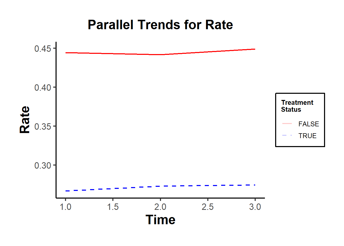

Figure 35.27: Parallel trends for the rate outcome between California and control units.

# do it manually
# always good but plot the dependent out
od |>
    # group by treatment status and time
    dplyr::group_by(California, Quarter) |>
    dplyr::summarize_all(mean) |>
    dplyr::ungroup() |>
    # view()
    
    ggplot2::ggplot(aes(x = Quarter_Num, y = Rate, color = California)) +
    ggplot2::geom_line() +
    causalverse::ama_theme()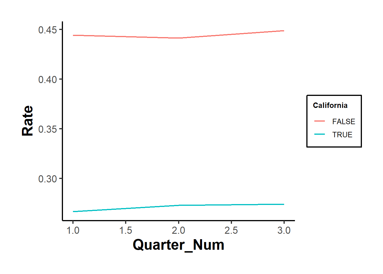

Figure 35.28: Manual parallel trends plot showing average rates.

Figures 35.27 and 35.28 show the raw outcomes by periods, while Figure 35.29 shows their coefficient estimates’ version.

# but it's also important to use statistical test
prior_trend <- fixest::feols(Rate ~ i(Quarter_Num, California) |
                                 State + Quarter,
                             data = od)

fixest::coefplot(prior_trend, grid = F)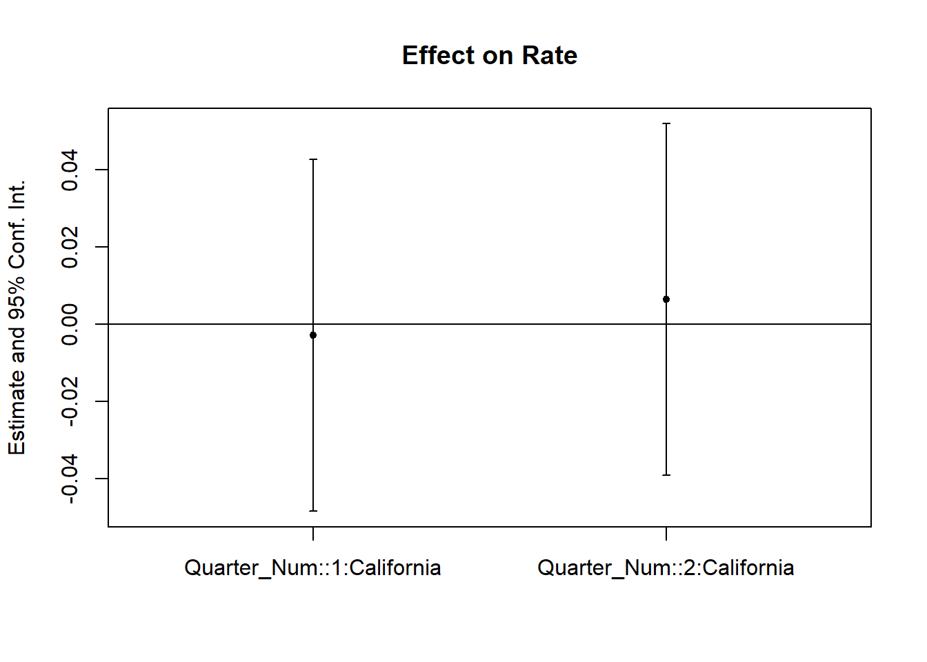

Figure 35.29: Coefficient plot for the prior-trend analysis.

# fixest::iplot(prior_trend, grid = F)

If one of the periods is significantly different from 0, our parallel trends assumption is not plausible.

In cases where the parallel trends assumption is questionable, researchers should consider methods for assessing and addressing potential violations. Some key approaches are discussed in Rambachan and Roth (2023):

• Imposing Restrictions: Constrain how different the post-treatment violations of parallel trends can be relative to pre-treatment deviations.

• Partial Identification: Rather than assuming a single causal effect, derive bounds on the ATT.

• Sensitivity Analysis: Evaluate how sensitive the results are to potential deviations from parallel trends.

To implement these approaches, the HonestDiD package by Rambachan and Roth (2023) provides robust statistical tools:

# https://github.com/asheshrambachan/HonestDiD
# remotes::install_github("asheshrambachan/HonestDiD")
# library(HonestDiD)

Alternatively, Ban and Kedagni (2022) propose a method that incorporates pre-treatment covariates as an information set and makes an assumption about the selection bias in the post-treatment period. Specifically, they assume that the selection bias lies within the convex hull of all pre-treatment selection biases. Under this assumption:

• They identify a set of possible ATT values.

• With a stronger assumption on selection bias, grounded in policymakers’ perspectives, they can estimate a point estimate of ATT.

Another useful tool for assessing parallel trends is the pretrends package by Roth (2022), which provides formal pre-trend tests:

# Install and load the pretrends package
# install.packages("pretrends")
# library(pretrends)

---

35.15.2 Placebo Test

A placebo test is a diagnostic tool used in Difference-in-Differences analysis to assess whether the estimated treatment effect is driven by pre-existing trends rather than the treatment itself. The idea is to estimate a treatment effect in a scenario where no actual treatment occurred. If a significant effect is found, it suggests that the parallel trends assumption may not hold, casting doubt on the validity of the causal inference.

Placebo tests sit alongside the prior parallel-trends test in a complementary role: where the event-study test asks whether deviations are visible in the data we have, the placebo test asks whether the estimator generates spurious effects when the treatment label is moved to a unit or period where, by construction, no causal effect can exist. A clean event study without a clean placebo is suggestive but unsatisfying, and a clean placebo with a noisy event study is harder to dismiss than the raw \(p\)-values alone would imply. Treating the two as a pair helps build the kind of layered defense of parallel trends that complements the partial-identification analysis later in this chapter.

Types of Placebo DiD Tests

1. Group-Based Placebo Test

• Assign treatment to a group that was never actually treated and rerun the DiD model.
• If the estimated treatment effect is statistically significant, this suggests that differences between groups, not the treatment, are driving results.
• This test helps rule out the possibility that the estimated effect is an artifact of unobserved systematic differences.

A valid treatment effect should be consistent across different reasonable control groups. To assess this:

• Rerun the DiD model using an alternative but comparable control group.

• Compare the estimated treatment effects across multiple control groups.

• If results vary significantly, this suggests that the choice of control group may be influencing the estimated effect, indicating potential selection bias or unobserved confounding.

2. Time-Based Placebo Test

• Conduct DiD using only pre-treatment data, pretending that treatment occurred at an earlier period.
• A significant estimated treatment effect implies that differences in pre-existing trends, not treatment, are responsible for observed post-treatment effects.
• This test is particularly useful when concerns exist about unobserved shocks or anticipatory effects.

Random Reassignment of Treatment

• Keep the same treatment and control periods but randomly assign treatment to units that were not actually treated.
• If a significant DiD effect still emerges, it suggests the presence of biases, unobserved confounding, or systematic differences between groups that violate the parallel trends assumption.

---

Procedure for a Placebo Test

1. Using Pre-Treatment Data Only

A robust placebo test often involves analyzing only pre-treatment periods to check whether spurious treatment effects appear. The procedure includes:

• Restricting the sample to pre-treatment periods only.

• Assigning a fake treatment period before the actual intervention.

• Testing a sequence of placebo cutoffs over time to examine whether different assumed treatment timings yield significant effects.

• Generating random treatment periods and using randomization inference to assess the sampling distribution of the placebo effect.

• Estimating the DiD model using the fake post-treatment period (post_time = 1).

• Interpretation: If the estimated treatment effect is statistically significant, this indicates that pre-existing trends (not treatment) might be influencing results, violating the parallel trends assumption.

2. Using Control Groups for a Placebo Test

If multiple control groups are available, a placebo test can also be conducted by:

• Dropping the actual treated group from the analysis.

• Assigning one of the control groups as a fake treated group.

• Estimating the DiD model and checking whether a significant effect is detected.

• Interpretation:

  • If a placebo effect appears (i.e., the estimated treatment effect is significant), it suggests that even among control groups, systematic differences exist over time.

  • However, this result is not necessarily disqualifying. Some methods, such as Synthetic Control, explicitly model such differences while maintaining credibility.

---

# Load necessary libraries
library(tidyverse)
library(fixest)
library(ggplot2)
library(causaldata)

# Load the dataset
od <- causaldata::organ_donations %>%
    # Use only pre-treatment data
    dplyr::filter(Quarter_Num <= 3) %>%
    
    # Create fake (placebo) treatment variables
    dplyr::mutate(
        FakeTreat1 = as.integer(State == 'California' &
                                    Quarter %in% c('Q12011', 'Q22011')),
        FakeTreat2 = as.integer(State == 'California' &
                                    Quarter == 'Q22011')
    )

# Estimate the placebo effects using fixed effects regression
clfe1 <- fixest::feols(Rate ~ FakeTreat1 | State + Quarter, data = od)
clfe2 <- fixest::feols(Rate ~ FakeTreat2 | State + Quarter, data = od)

# Display the regression results
fixest::etable(clfe1, clfe2)
#>                           clfe1            clfe2
#> Dependent Var.:            Rate             Rate
#>                                                 
#> FakeTreat1      0.0061 (0.0195)                 
#> FakeTreat2                      -0.0017 (0.0195)
#> Fixed-Effects:  --------------- ----------------
#> State                       Yes              Yes
#> Quarter                     Yes              Yes
#> _______________ _______________ ________________
#> S.E. type                   IID              IID
#> Observations                 81               81
#> R2                      0.99377          0.99376
#> Within R2               0.00192          0.00015
#> ---
#> Signif. codes: 0 '***' 0.001 '**' 0.01 '*' 0.05 '.' 0.1 ' ' 1

# Extract coefficients and confidence intervals
coef_df <- tibble(
    Model = c("FakeTreat1", "FakeTreat2"),
    Estimate = c(coef(clfe1)["FakeTreat1"], coef(clfe2)["FakeTreat2"]),
    SE = c(summary(clfe1)$coeftable["FakeTreat1", "Std. Error"], 
           summary(clfe2)$coeftable["FakeTreat2", "Std. Error"]),
    Lower = Estimate - 1.96 * SE,
    Upper = Estimate + 1.96 * SE
)

# Plot the placebo effects
ggplot(coef_df, aes(x = Model, y = Estimate)) +
    geom_point(size = 3, color = "blue") +
    geom_errorbar(aes(ymin = Lower, ymax = Upper), width = 0.2, color = "blue") +
    geom_hline(yintercept = 0, linetype = "dashed", color = "red") +
    theme_minimal() +
    labs(
        title = "Placebo Treatment Effects",
        y = "Estimated Effect on Organ Donation Rate",
        x = "Placebo Treatment"
    )

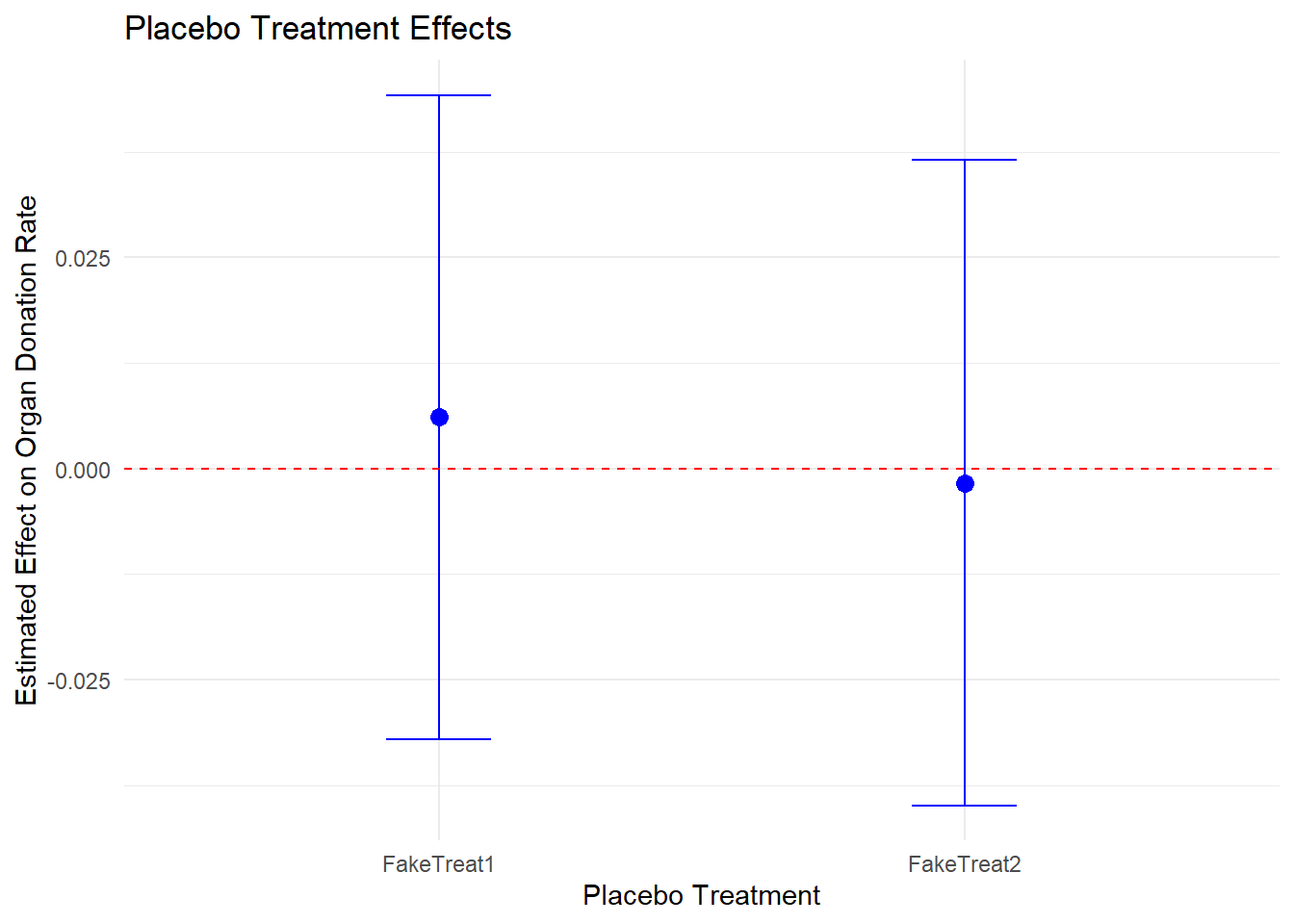
Figure 35.30: Placebo treatment effects on organ donation rate.

We would like the “supposed” DiD to be insignificant (Figure 35.30).

35.16 Robustness Checks

A well-executed Difference-in-Differences analysis requires robustness checks to verify the validity of estimated treatment effects and best practices to ensure methodological rigor. Whereas the prior parallel-trends test and the placebo test interrogate the identifying assumption, the checks below interrogate the modeling choices layered on top of it: the time window, the functional form for trends, the choice of outcome, and the inclusion of an additional comparison dimension via triple differences. Stability of the estimate across these choices is what allows a reader to attribute the result to the policy variation rather than to a fortunate specification. The broader catalog of robustness checks for quasi-experimental designs and the discussion of coefficient stability bounds elsewhere in the book extend the same logic.

---

35.16.1 Robustness Checks to Strengthen Causal Interpretation

Once the parallel trends assumption is assessed, additional robustness tests ensure that treatment effects are not driven by confounding factors or modeling choices.

1. Varying the Time Window

• Shorter time windows reduce exposure to long-term confounders but risk losing statistical power.
• Longer time windows capture persistent effects but may introduce unrelated policy changes.
• Solution: Estimate the DiD model across different time horizons and check if results are stable.

2. Higher-Order Polynomial Time Trends

• Standard DiD models assume a linear time trend.
• If trends are nonlinear, this assumption may be too restrictive.
• Solution: Introduce quadratic or cubic time trends and verify whether results hold.

3. Testing Alternative Dependent Variables

• The treatment should only affect the expected dependent variable.
• A robustness check involves running the DiD on unrelated dependent variables.
• If treatment effects appear where they should not, this signals a possible identification problem.

4. Triple-Difference (DDD) Strategy

A Triple-Difference (DDD) model adds an additional comparison group to address remaining biases:

\[ \begin{aligned} Y_{ijt} &= \alpha + \gamma Treat_{i} + \lambda Post_t + \theta Group_j + \delta_1 (Treat_i \times Post_t) \\ &+ \delta_2 (Treat_i \times Group_j) + \delta_3 (Post_t \times Group_j) \\ &+ \delta_4 (Treat_i \times Post_t \times Group_j) + \epsilon_{ijt} \end{aligned} \]

where:

• \(Group_j\) represents a subgroup within treatment/control (e.g., high- vs. low-intensity exposure).

• \(\delta_4\) captures the DDD effect, which removes residual biases present in the standard DiD model.

---

35.16.2 Best Practices for Reliable DiD Implementation

To improve the credibility and transparency of DiD estimates, researchers should adhere to the following best practices:

1. Documenting Treatment Cohorts

• Clearly report the number of treated and control units over time.
• If treatment is staggered, adjust for different exposure durations.

2. Checking Covariate Balance & Overlap

• Verify whether the distribution of covariates is similar across treatment and control groups.
• If treatment and control groups differ significantly, consider using matching methods.

3. Conducting Sensitivity Analyses for Parallel Trends

• Apply alternative weighting schemes (e.g., entropy balancing) to reduce dependence on model assumptions.
• Use honestDiD to test robustness under different parallel trends violations.

35.17 Concerns in DID

The catalogue below collects the issues that recur most often in applied work and pairs each with the diagnostic or estimator that addresses it. Several of them (heterogeneous effects, treatment timing, questionable counterfactuals) feed directly into the modern staggered-adoption literature in Section 35.12; others (selection on unobservables, Ashenfelter’s dip) connect more naturally to Rosenbaum bounds and to the broader conditional ignorability discussion. The point is not that every analysis must address every concern, but that a credible DiD application explicitly considers which of them are plausible in the context at hand and chooses diagnostics accordingly.

35.17.1 Limitations and Common Issues

1. Functional Form Dependence

• If the response to treatment is nonlinear, compare high- vs. low-intensity groups.

2. Selection on (Time-Varying) Unobservables

• Use Rosenbaum Bounds to check the sensitivity of estimates to unobserved confounders.

3. Long-Term Effects

• Parallel trends are more reliable in short time windows.
• Over long periods, other confounding factors may emerge.

4. Heterogeneous Effects

• Treatment intensity (e.g., different doses) may vary across groups, leading to different effects.

5. Ashenfelter’s Dip (Ashenfelter 1978)

• Participants in job training programs often experience earnings drops before enrolling, making them systematically different from nonparticipants.
• Fix: Compute long-run differences, excluding periods around treatment, to test for sustained impact (Proserpio and Zervas 2017; Heckman et al. 1999; Jepsen et al. 2014).

6. Lagged Treatment Effects

• If effects are not immediate, using a lagged dependent variable \(Y_{it-1}\) may be more appropriate (Blundell and Bond 1998).

7. Bias from Unobserved Factors Affecting Trends

• If external shocks influence treatment and control groups differently, this biases DiD estimates.

8. Correlated Observations

• Standard errors should be clustered appropriately.

9. Incidental Parameters Problem (Lancaster 2000)

• Always prefer individual and time fixed effects to reduce bias.

10. Treatment Timing and Negative Weights

• If treatment timing varies across units, negative weights can arise in standard DiD estimators when treatment effects are heterogeneous (Athey and Imbens 2022; Borusyak et al. 2024; Goodman-Bacon 2021). The Goodman-Bacon decomposition is the standard diagnostic for the presence and severity of these forbidden comparisons.
• Fix: Use estimators from Callaway and Sant’Anna (2021) and De Chaisemartin and d’Haultfoeuille (2020) (did package). Specifically, the group-time ATT estimator and the switching-DiD estimator avoid the contaminated comparisons that produce negative weights, and the stacked DiD design provides a transparent alternative when the analyst prefers to keep a single regression.
• If expecting lags and leads, see Sun and Abraham (2021), whose cohort ATT approach generalizes naturally to event-study settings.

11. Treatment Effect Heterogeneity Across Groups

• If treatment effects vary across groups and interact with treatment variance, standard estimators may be invalid (Gibbons et al. 2018). Beyond the staggered-adoption tools above, the reshaped IPW TWFE estimator and the matrix-completion estimator are useful when heterogeneity is suspected to load on covariates or on idiosyncratic unit-time shocks rather than purely on cohort.

12. Endogenous Timing

If the timing of units can be influenced by strategic decisions in a DID analysis, an instrumental variable approach with a control function can be used to control for endogeneity in timing. See Section 39 for the IV machinery and Section 31.7.1 for design-based alternatives.

13. Questionable Counterfactuals

In situations where the control units may not serve as a reliable counterfactual for the treated units, matching methods such as propensity score matching or generalized random forest can be utilized. Additional methods can be found in Matching Methods. When parallel trends in levels is implausible but the treated unit can be approximated by a weighted combination of controls, synthetic control and the hybrid synthetic DiD approach are natural fallbacks; the panel-match estimator and the family of counterfactual estimators extend the idea to richer treatment-history settings.

35.17.2 Matching Methods in DID

Matching methods are often used in causal inference to balance treated and control units based on pre-treatment observables. In the context of Difference-in-Differences, matching helps:

• Reduce selection bias by ensuring that treated and control units are comparable before treatment.
• Improve parallel trends validity by selecting control units with similar pre-treatment trajectories.
• Enhance robustness when treatment assignment is non-random across groups.

Key Considerations in Matching

• Standard Errors Need Adjustment
  • Standard errors should account for the fact that matching reduces variance (Heckman et al. 1997).
  • A more robust alternative is Doubly Robust DID (Sant’Anna and Zhao 2020), where either matching or regression suffices for unbiased treatment effect identification.
• Group Fixed Effects Alone Do Not Eliminate Selection Bias
  • Fixed effects absorb time-invariant heterogeneity, but do not correct for selection into treatment.
  • Matching helps close the “backdoor path” between:
    1. Propensity to be treated
    2. Dynamics of outcome evolution post-treatment
• Matching on Time-Varying Covariates
  • Beware of regression to the mean: extreme pre-treatment outcomes may artificially bias post-treatment estimates (Daw and Hatfield 2018).
  • This issue is less concerning for time-invariant covariates.
• Comparing Matching vs. DID Performance
  • Matching and DID both use pre-treatment outcomes to mitigate selection bias.
  • Simulations (Chabé-Ferret 2015) show that:
    • Matching tends to underestimate the true treatment effect but improves with more pre-treatment periods.
    • When selection bias is symmetric, Symmetric DID (equal pre- and post-treatment periods) performs well.
    • When selection bias is asymmetric, DID generally outperforms Matching.
• Forward DID as a Control Unit Selection Algorithm
  • An efficient way to select control units is Forward DID (Li 2024).

---

35.17.3 Control Variables in DID

• Always report results with and without controls:
  • If controls are fixed within groups or time periods, they should be absorbed in fixed effects.
  • If controls vary across both groups and time, this suggests the parallel trends assumption is questionable.
• \(R^2\) is not crucial in causal inference:
  • Unlike predictive models, causal models do not prioritize explanatory power (\(R^2\)), but rather unbiased identification of treatment effects.

---

35.17.4 DID for Count Data: Fixed-Effects Poisson Model

For count data, one can use the fixed-effects Poisson pseudo-maximum likelihood estimator (PPML) (Athey and Imbens 2006; Puhani 2012). Applications of this method can be found in management (Burtch et al. 2018) and marketing (He et al. 2021).

This approach offers robust standard errors under over-dispersion (Wooldridge 1999) and is particularly useful when dealing with excess zeros in the data.

Key advantages of PPML:

• Handles zero-inflated data better than log-OLS: A log-OLS regression may produce biased estimates (O’Hara and Kotze 2010) when heteroskedasticity is present (Silva and Tenreyro 2006), especially in datasets with many zeros (Silva and Tenreyro 2011).
• Avoids the limitations of negative binomial fixed effects: Unlike Poisson, there is no widely accepted fixed-effects estimator for the negative binomial model (Allison and Waterman 2002).

---

35.17.5 Handling Zero-Valued Outcomes in DID

Zero-valued outcomes are a special case of the broader functional-form sensitivity that runs through this chapter. In the canonical DiD model, parallel trends is a property of the outcome scale, so transforming the outcome (logs, percent changes, normalized counts) silently changes the identifying assumption being made. When a non-trivial fraction of the data is at zero, the choice of scale also collides with the distinction between intensive- and extensive-margin responses. The two approaches below take different stances on that tradeoff, and they should be read alongside the changes-in-changes estimator, which provides a fully nonparametric alternative when the analyst is unwilling to commit to either parallel trends in levels or parallel trends in ratios.

When dealing with zero-valued outcomes, it is crucial to separate the intensive margin effect (e.g., outcome changes from 10 to 11) from the extensive margin effect (e.g., outcome changes from 0 to 1).

A common issue is that the treatment coefficient from a log-transformed regression cannot be directly interpreted as a percentage change when zeros are present (Chen and Roth 2024). To address this, we can consider two alternative approaches:

1. Proportional Treatment Effects

We define the percentage change in the treated group’s post-treatment outcome as:

\[ \theta_{ATT\%} = \frac{E[Y_{it}(1) \mid D_i = 1, Post_t = 1] - E[Y_{it}(0) \mid D_i = 1, Post_t = 1]}{E[Y_{it}(0) \mid D_i = 1, Post_t = 1]} \]

Instead of assuming parallel trends in levels, we can rely on a parallel trends assumption in ratios (Wooldridge 2023).

The Poisson QMLE model is:

\[ Y_{it} = \exp(\beta_0 + \beta_1 D_i \times Post_t + \beta_2 D_i + \beta_3 Post_t + X_{it}) \epsilon_{it} \]

The treatment effect is estimated as:

\[ \hat{\theta}_{ATT\%} = \exp(\hat{\beta}_1) - 1 \]

To validate the parallel trends in ratios assumption, we can estimate a dynamic Poisson QMLE model:

\[ Y_{it} = \exp(\lambda_t + \beta_2 D_i + \sum_{r \neq -1} \beta_r D_i \times (RelativeTime_t = r)) \]

If the assumption holds, we expect:

\[ \exp(\hat{\beta}_r) - 1 = 0 \quad \text{for} \quad r < 0. \]

Even if the pre-treatment estimates appear close to zero, we should still conduct a sensitivity analysis (Rambachan and Roth 2023) to assess robustness (see Prior Parallel Trends Test).

library(fixest)

base_did_log0 <- base_did |> 
    mutate(y = if_else(y > 0, y, 0))

res_pois_es <-
    fepois(y ~ x1 + i(period, treat, 5) | id + period,
           data = base_did_log0,
           vcov = "hetero")

etable(res_pois_es)
#>                            res_pois_es
#> Dependent Var.:                      y
#>                                       
#> x1                  0.1895*** (0.0108)
#> treat x period = 1    -0.2769 (0.3545)
#> treat x period = 2    -0.2699 (0.3533)
#> treat x period = 3     0.1737 (0.3520)
#> treat x period = 4    -0.2381 (0.3249)
#> treat x period = 6     0.3724 (0.3086)
#> treat x period = 7    0.7739* (0.3117)
#> treat x period = 8    0.5028. (0.2962)
#> treat x period = 9   0.9746** (0.3092)
#> treat x period = 10  1.310*** (0.3193)
#> Fixed-Effects:      ------------------
#> id                                 Yes
#> period                             Yes
#> ___________________ __________________
#> S.E. type           Heteroskedas.-rob.
#> Observations                     1,080
#> Squared Cor.                   0.51131
#> Pseudo R2                      0.34836
#> BIC                            5,868.8
#> ---
#> Signif. codes: 0 '***' 0.001 '**' 0.01 '*' 0.05 '.' 0.1 ' ' 1

Figure 35.31 shows the parallel trends before treatment and the effect after treatment.

iplot(res_pois_es)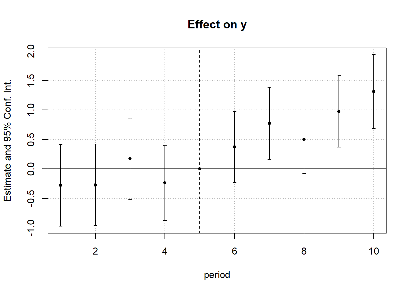

Figure 35.31: Event-study estimates from a Poisson regression model.

This parallel trend is the “ratio” version as in Wooldridge (2023) :

\[ \frac{E(Y_{it}(0) |D_i = 1, Post_t = 1)}{E(Y_{it}(0) |D_i = 1, Post_t = 0)} = \frac{E(Y_{it}(0) |D_i = 0, Post_t = 1)}{E(Y_{it}(0) |D_i =0, Post_t = 0)} \]

which means without treatment, the average percentage change in the mean outcome for treated group is identical to that of the control group.

2. Log Effects with Calibrated Extensive-Margin Value

A potential limitation of proportional treatment effects is that they may not be well-suited for heavy-tailed outcomes. In such cases, we may prefer to explicitly model the extensive margin effect.

Following (Chen and Roth 2024, 39), we can calibrate the weight placed on the intensive vs. extensive margin to ensure meaningful interpretation of the treatment effect.

If we want to study the treatment effect on a concave transformation of the outcome that is less influenced by those in the distribution’s tail, then we can perform this analysis.

Steps:

1. Normalize the outcomes such that 1 represents the minimum non-zero and positive value (i.e., divide the outcome by its minimum non-zero and positive value).
2. Estimate the treatment effects for the new outcome

\[ m(y) = \begin{cases} \log(y) & \text{for } y >0 \\ -x & \text{for } y = 0 \end{cases} \]

The choice of \(x\) depends on what the researcher is interested in:

Value of \(x\)	Interest
\(x = 0\)	The treatment effect in logs where all zero-valued outcomes are set to equal the minimum non-zero value (i.e., we exclude the extensive-margin change between 0 and \(y_{min}\) )
\(x>0\)	Setting the change between 0 and \(y_{min}\) to be valued as the equivalent of a \(x\) log point change along the intensive margin.

library(fixest)
base_did_log0_cali <- base_did_log0 |> 
    # get min 
    mutate(min_y = min(y[y > 0])) |> 
    
    # normalized the outcome 
    mutate(y_norm = y / min_y)

my_regression <-
    function(x) {
        base_did_log0_cali <-
            base_did_log0_cali %>% mutate(my = ifelse(y_norm == 0,-x,
                                                      log(y_norm)))
        my_reg <-
            feols(
                fml = my ~ x1 + i(period, treat, 5) | id + period,
                data = base_did_log0_cali,
                vcov = "hetero"
            )
        
        return(my_reg)
    }

xvec <- c(0, .1, .5, 1, 3)
reg_list <- purrr::map(.x = xvec, .f = my_regression)


iplot(reg_list, 
      pt.col =  1:length(xvec),
      pt.pch = 1:length(xvec))
legend("topleft", 
       col = 1:length(xvec),
       pch = 1:length(xvec),
       legend = as.character(xvec))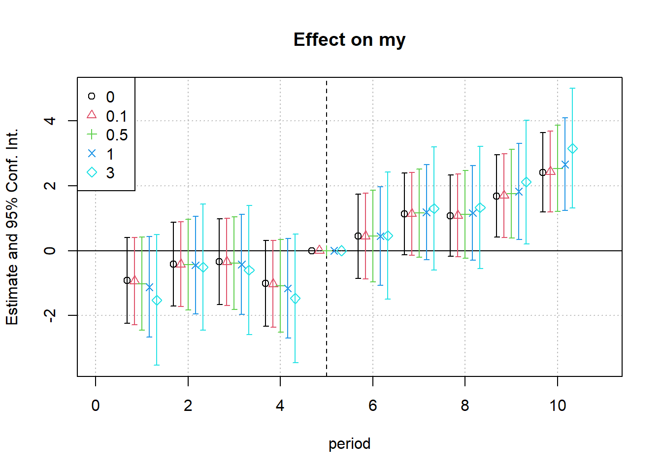

etable(
    reg_list,
    headers = list("Extensive-margin value (x)" = as.character(xvec)),
    digits = 2,
    digits.stats = 2
)
#>                                   model 1        model 2        model 3
#> Extensive-margin value (x)              0            0.1            0.5
#> Dependent Var.:                        my             my             my
#>                                                                        
#> x1                         0.43*** (0.02) 0.44*** (0.02) 0.46*** (0.03)
#> treat x period = 1           -0.92 (0.67)   -0.94 (0.69)    -1.0 (0.73)
#> treat x period = 2           -0.41 (0.66)   -0.42 (0.67)   -0.43 (0.71)
#> treat x period = 3           -0.34 (0.67)   -0.35 (0.68)   -0.38 (0.73)
#> treat x period = 4            -1.0 (0.67)    -1.0 (0.68)    -1.1 (0.73)
#> treat x period = 6            0.44 (0.66)    0.44 (0.67)    0.45 (0.72)
#> treat x period = 7            1.1. (0.64)    1.1. (0.65)    1.2. (0.70)
#> treat x period = 8            1.1. (0.64)    1.1. (0.65)     1.1 (0.69)
#> treat x period = 9           1.7** (0.65)   1.7** (0.66)    1.8* (0.70)
#> treat x period = 10         2.4*** (0.62)  2.4*** (0.63)  2.5*** (0.68)
#> Fixed-Effects:             -------------- -------------- --------------
#> id                                    Yes            Yes            Yes
#> period                                Yes            Yes            Yes
#> __________________________ ______________ ______________ ______________
#> S.E. type                  Heterosk.-rob. Heterosk.-rob. Heterosk.-rob.
#> Observations                        1,080          1,080          1,080
#> R2                                   0.43           0.43           0.43
#> Within R2                            0.26           0.26           0.25
#> 
#>                                   model 4        model 5
#> Extensive-margin value (x)              1              3
#> Dependent Var.:                        my             my
#>                                                         
#> x1                         0.49*** (0.03) 0.62*** (0.04)
#> treat x period = 1            -1.1 (0.79)     -1.5 (1.0)
#> treat x period = 2           -0.44 (0.77)   -0.51 (0.99)
#> treat x period = 3           -0.43 (0.78)    -0.60 (1.0)
#> treat x period = 4            -1.2 (0.78)     -1.5 (1.0)
#> treat x period = 6            0.45 (0.77)     0.46 (1.0)
#> treat x period = 7             1.2 (0.75)     1.3 (0.97)
#> treat x period = 8             1.2 (0.74)     1.3 (0.96)
#> treat x period = 9            1.8* (0.75)    2.1* (0.97)
#> treat x period = 10         2.7*** (0.73)  3.2*** (0.94)
#> Fixed-Effects:             -------------- --------------
#> id                                    Yes            Yes
#> period                                Yes            Yes
#> __________________________ ______________ ______________
#> S.E. type                  Heterosk.-rob. Heterosk.-rob.
#> Observations                        1,080          1,080
#> R2                                   0.42           0.41
#> Within R2                            0.25           0.24
#> ---
#> Signif. codes: 0 '***' 0.001 '**' 0.01 '*' 0.05 '.' 0.1 ' ' 1

We have the dynamic treatment effects for different hypothesized extensive-margin value of \(x \in (0, .1, .5, 1, 3, 5)\)

The first column is when the zero-valued outcome equal to \(y_{min, y>0}\) (i.e., there is no difference between the minimum outcome and zero outcome - \(x = 0\))

For this particular example, as the extensive margin increases, we see an increase in the effect magnitude. The second column is when we assume an extensive-margin change from 0 to \(y_{min, y >0}\) is equivalent to a 10 (i.e., \(0.1 \times 100\)) log point change along the intensive margin.

---

35.17.6 Standard Errors

One of the major statistical challenges in DiD estimation is serial correlation in the error terms. This issue is particularly problematic because it can lead to underestimated standard errors, inflating the likelihood of Type I errors (false positives). As discussed in Bertrand et al. (2004), serial correlation arises in DiD settings due to several factors:

1. Long time series: Many DiD studies use multiple time periods, increasing the risk of correlated errors.
2. Highly positively serially correlated outcomes: Many economic and business variables (e.g., GDP, sales, employment rates) exhibit strong persistence over time.
3. Minimal within-group variation in treatment timing: For example, in a state-level policy change, all individuals in a state receive treatment at the same time, leading to correlation within state-time clusters.

To correct for serial correlation, various methods can be employed. However, some approaches work better than others:

• Avoid standard parametric corrections: A common approach is to model the error term using an autoregressive (AR) process. However, Bertrand et al. (2004) show that this often fails in DiD settings because it does not fully account for within-group correlation.
• Nonparametric solutions (preferred when the number of groups is large):
  • Block bootstrap: Resampling entire groups (e.g., states) rather than individual observations maintains the correlation structure and provides robust standard errors.
• Collapsing data into two periods (Pre vs. Post):
  • Aggregating the data into a single pre-treatment and single post-treatment period can mitigate serial correlation issues. This approach is particularly useful when the number of groups is small (Donald and Lang 2007).
  • Note: While this reduces the power of the analysis by discarding variation across time, it ensures that standard errors are not artificially deflated.
• Variance-covariance matrix corrections:
  • Empirical corrections (e.g., cluster-robust standard errors) and arbitrary variance-covariance matrix adjustments (e.g., Newey-West) can work well, but they are reliable only in large samples.

Overall, selecting the appropriate correction method depends on the sample size and structure of the data. When possible, block bootstrapping and collapsing data into pre/post periods are among the most effective approaches. The serial-correlation problem is also one of the reasons that modern staggered-adoption estimators (Section 35.12) report cluster-bootstrap standard errors by default, and it is closely connected to the inference issues flagged in the SUTVA discussion when treatment exposure is correlated within clusters.

---

35.17.7 Partial Identification

Classical DiD delivers a point-identified estimate of the average treatment effect on the treated (ATT) only when the parallel-trends assumption is exact. Yet in practice pre-trends often deviate or post-treatment shocks differ across groups (e.g., the famous Ashenfelter (1978)). Partial-identification (PI) methods shift the question from “Is the estimate unbiased?” to “How much would the identifying assumption have to fail before I reverse my conclusion?”

In the diagnostic workflow sketched at the start of this chapter, partial identification is the natural last line of defense once the visual checks, event-study tests, and placebo tests have all left some residual doubt. It is also the right tool when pre-trend tests are statistically silent but underpowered: rather than treating “we failed to reject” as proof of parallel trends, the analyst reports the magnitude of violation that the data would still permit. Used this way, PI complements the heterogeneity-robust estimators in Section 35.12 and the coefficient stability bounds machinery: the former handles bias from contaminated comparisons, while PI handles bias from a violated identifying assumption itself.

The partial-identification literature that has grown up around DiD reflects a series of distinct philosophical bets about how to make the “how much could parallel trends fail?” question precise. It is helpful to walk through them in order, because each one chooses a different lever to constrain.

The starting point is Manski and Pepper (2018), who simply ask the analyst to commit to any substantively credible bounds on \(\delta\), across time, across space, or both, and then propagate those bounds through to the ATT. The approach is conceptually clean but requires the researcher to defend the bounds from outside the data. L. J. Keele et al. (2019) sharpen the question into something more empirically tractable by importing Rosenbaum-style sensitivity analysis from the matching literature: rather than bounding \(\delta\) directly, fix a single sensitivity parameter that measures how much hidden bias one would need to reverse the estimated sign. L. Keele et al. (2019) extend this machinery to compound treatments, where the treated group is simultaneously exposed to another event, asking whether the causal claim survives under that more demanding scenario.

A different strategy is to lean on auxiliary control groups rather than auxiliary parameters. Ye et al. (2024) use two control groups exposed to negatively correlated shocks to non-parametrically bracket the counterfactual trend, sidestepping parallel trends without committing to a specific bound on \(\delta\). Leavitt (2020) goes Bayesian: a hierarchical prior shrinks extreme violations of parallel trends and yields credible intervals that account for trend heterogeneity directly.

The most influential synthesis is Rambachan and Roth (2023), which collapses the question into a researcher-chosen smoothness or magnitude restriction and then reports the breakdown threshold, the value of the restriction at which the confidence set first touches zero. Two bounding strategies fall out of this framework, both implemented in the honestdid package and discussed in detail later in this section: relative-magnitude bounds, which constrain \(|\delta|\) to be no larger than \(M\) times the worst pre-period jump, and smoothness bounds, which allow the slope of \(\delta\) to shift by at most \(M\) per period.

---

35.17.7.1 Canonical DiD notation and the source of bias

Let

• \(Y_{it}^{1}\) and \(Y_{it}^{0}\) be potential outcomes for unit \(i\) in period \(t\) under treatment and no treatment;
• \(D_i\in{0,1}\) indicate ever-treated units;
• \(\texttt{Post}_t\) mark periods after the policy shock.

For two periods (pre, post) and two groups (T = treated, U = untreated) the simple DiD estimator is

\[ \hat\beta_{DD}= \left[E(Y_T^{1}\mid \texttt{Post})-E(Y_T^{0}\mid \texttt{Pre})\right]-\left[E(Y_U^{0}\mid \texttt{Post})-E(Y_U^{0}\mid \texttt{Pre})\right] \]

Add and subtract the counterfactual trend \(E(Y_T^{0}\mid \texttt{Post})\) and rearrange:

\[ \begin{aligned} \hat\beta_{DD} &= \underbrace{E(Y_T^{1}\mid\texttt{Post})-E(Y_T^{0}\mid\texttt{Post})}_{\text{ATT}} \\ &+ \underbrace{[E(Y_T^{0}\mid\texttt{Post})-E(Y_T^{0}\mid\texttt{Pre})] -[E(Y_U^{0}\mid\texttt{Post})-E(Y_U^{0}\mid\texttt{Pre})]}_{\delta} \end{aligned} \]

Hence

\[ \hat\beta_{DD}= \text{ATT}+\delta . \]

When parallel trends hold, \(\delta=0\); any violation translates one-for-one into bias (Frake et al. 2025).

---

35.17.7.2 Bounding the ATT when \(\delta\neq 0\)

The core PI idea is simple: derive credible bounds on \(\delta\), then translate those into bounds on the ATT.

Two families of restrictions, both operationalized by Rambachan and Roth (2023) and implemented in the honestdid package, are now widely used:

1. Relative-magnitude (RM) bounds: the post-treatment gap \(|\delta|\) cannot exceed \(M\) times the largest period-to-period deviation observed in the pre-treatment event-study.
2. Smoothness (SM) bounds: the slope of the treated-minus-control gap can change by at most \(M\) units each period after treatment.

Because \(M\) is researcher-chosen, inference is reported across a grid of plausible \(M\) values, revealing the breakdown threshold where the confidence set first touches zero (Frake et al. 2025, 14).

---

35.17.7.3 Relative-Magnitude Restriction

Let \(\hat g_t\) be the event-study coefficient at time \(t\) (normalized to zero at \(t=-1\)).

• Step 1: calibrate the worst pre-trend:
  \(M_0 = \max_{s<0} |\hat g_s-\hat g_{s-1}|\).

• Step 2: allow proportional violations post-treatment:
  Impose \(|\delta_t|\le M\cdot M_0\) for every \(t\ge 0\).

• Step 3: construct “honest” confidence sets for the ATT or for period-specific effects by solving a constrained least-squares problem (Rambachan and Roth 2023).

---

35.17.7.4 Smoothness Restriction

When violations evolve gradually (e.g., treated units drift upward over time), the SM bound is more credible.

• Step 1: estimate the pre-treatment slope:
  \(s_0 = \hat g_{-1}-\hat g_{-2}\).

• Step 2: restrict post-treatment slopes:
  The counterfactual slope in period \(k\) may vary within
  \([s_0-M, s_0+M]\).

• Step 3: propagate forward to obtain an admissible path for \(\delta_t\); compute the least-favorable path, then derive confidence sets (Rambachan and Roth 2023).

---

35.17.7.5 Step-by-step Empirical Workflow

See Frake et al. (2025), p. 15 for a decision tree that guides the choice of method.

1. Graph the event-study. Are any pre-trends visible? Quantify their magnitude and/or slope.
2. Choose a restriction family (RM for episodic shocks, SM for trending deviations). Justify the choice theoretically (e.g., anticipation effects vs. gradual selection).
3. Select a grid of \(M\). Always display the break-even \(M^{*}\) where the CI first covers zero; interpret \(M^{*}\) in real-world units.
4. Report the full set, not only the “robust” interval. Transparency trumps opportunistic suppression.
5. Complement with falsification tests (placebo policy dates, placebo outcomes) to discipline the plausible range of \(M\).
6. Document software and code. honestdid (R/Stata) includes convenient wrappers for both restrictions and automatic figures.

---

35.17.7.6 Worked Example (Stylized)

Suppose pre-policy trends exhibit at most a 0.8-point swing. Setting \(M\in{0,0.5,1,1.5}\):

\(M\)	95 % CI for ATT	Conclusion
0	[0.85, 1.25]	Positive, robust
0.5	[0.60, 1.50]	Positive
1	[-0.05, 1.85]	Sign flips plausible
1.5	[-0.45, 2.25]	Cannot rule out zero

Thus the causal claim survives unless the unobserved counterfactual deviations are \(\ge 1 \times\) the worst pre-treatment kink, an interpretation far clearer than a single \(p\)-value.

---

35.17.7.7 Common Pitfalls and Best Practices

• Mistaking absence of significant pre-trends for proof of parallel-trends. Under-powered tests can miss economically large differences.
• Choosing \(M\) post-hoc. Decide the grid before looking at results.
• Ignoring sign. If theory predicts the treated counterfactual would have fallen, impose a one-sided bound; doing otherwise wastes power.
• Forgetting heterogeneous timing or staggered adoption. Apply PI to group-time ATT estimates from modern DiD estimators before aggregation.

Partial-identification transforms DiD from a “take-it-or-leave-it” enterprise into a transparent sensitivity analysis. By explicitly parameterizing and visually communicating, the extent of permissible departures from parallel trends, researchers allow readers to map their own priors onto empirical conclusions. Used thoughtfully, PI techniques enhance credibility without demanding the impossible.

---

35.17.7.8 Putting the Pieces Together

A defensible modern DiD analysis rarely relies on a single diagnostic; it layers several. A reasonable template, drawing on the tools surveyed in this chapter and on the broader quasi-experimental toolkit, looks like this. Begin with raw outcome plots and an event-study (the visualization and event studies sections give the mechanics) to inspect both levels and trends. If the data are staggered, run the Goodman-Bacon decomposition and re-estimate using a heterogeneity-robust estimator from Section 35.12 before drawing any substantive conclusion from a TWFE coefficient. Layer in placebo tests (group-based, time-based, and randomization-based) and the robustness checks above to discipline modeling choices. Where parallel trends in levels is suspect, consider matching, synthetic control, synthetic DiD, or changes-in-changes as design-level alternatives. Finally, use partial identification, with both relative-magnitude and smoothness restrictions, to communicate how much violation of the identifying assumption the conclusion can absorb. The point of the exercise is not to mechanically tick boxes but to give a reader a concrete sense of which failure modes have been ruled out, which remain plausible, and how much they would have to bite before the headline result reverses. A DiD analysis that survives that gauntlet is rarely “proven”, but it is unusually difficult to dismiss.

📖 Free preview — limited per publisher guidelines. Purchase the complete A Guide on Data Analysis series (Vols. 1–4) on Springer.

Vol. 1 Vol. 2 Vol. 3 Vol. 4