32 Synthetic Control

The Synthetic Control Method (SCM) is a powerful causal inference tool used when only one treated unit exists, and researchers must construct a synthetic comparison group from a donor pool of untreated units. Introduced by Abadie and Gardeazabal (2003) and later extended by Abadie, Diamond, and Hainmueller (2010), SCM has become a widely used method in policy evaluation and business analytics. See Abadie (2021) for a review of the method.

32.1 Why the method exists

The motivating problem is common in applied work. A single state passes a tax reform, a single firm rolls out a new pricing policy, a single country adopts a peg, and the analyst needs to estimate what would have happened in the absence of the intervention. With one treated unit, the comparison-group machinery of difference-in-differences is brittle: there is no obvious “control state” or “control firm” that constitutes a clean counterfactual, and any single donor selected is as much a research-design choice as the analysis itself. Synthetic control responds by replacing the judgment of a control with a construction: rather than selecting one comparable unit, the method builds a weighted average of many, where the weights are chosen so that the synthetic unit tracks the treated unit’s outcome and characteristics during the pre-treatment period as closely as possible. The treatment effect is then read off as the gap between the treated unit and its synthetic counterpart after the intervention.

The setting where this approach is most valuable is one in which (i) a clear and discrete policy event is to be evaluated, such as a minimum wage law, a tax reform, or a major advertising campaign, and (ii) there is essentially one unit on the treated side and several plausible controls on the other. Marketing and business applications have multiplied in exactly these settings. Tirunillai and Tellis (2017) use SCM to isolate the effect of offline TV advertising on online chatter; Wang, Wu, and Zhu (2019) estimate how mobile hailing technology shifted drivers’ hourly earnings; Guo, Sriram, and Manchanda (2020) evaluate the Massachusetts Open Payment Law’s effect on physician prescription behavior; and Adalja et al. (2023) exploit Vermont’s GMO-labeling law to ask whether mandatory disclosure changed consumer demand. Each of these has the SCM signature: one treated case, several donor candidates, and a sharp moment of intervention.

32.2 What the method buys you

The distinctive feature of SCM is not just that it provides an answer in this awkward setting, but what kind of answer it provides. Three properties are worth highlighting because they help explain the method’s appeal.

First, the construction is data-driven rather than judgment-driven. The donor pool’s weights are chosen by an optimization that minimizes pre-treatment fit; the analyst cannot tilt the comparison unit toward a preferred outcome. As Arkhangelsky and Hirshberg (2023) show, when the pre-treatment period is long enough, the resulting estimator delivers asymptotically normal parameters in linear panel models, putting it on the same theoretical footing as DiD.

Second, SCM matches on something stronger than covariates: it matches on pre-treatment outcomes. This is what distinguishes it from ordinary matching methods, which align units on \(X\) and rely on the unobservables to balance implicitly. By forcing the synthetic unit to track the treated unit’s outcome trajectory before treatment, SCM absorbs whatever combination of observed and unobserved factors generated that trajectory, at least to the extent they were operating in the donor pool. A Bayesian variant (Bayesian Synthetic Control) avoids the restrictive priors of the original formulation (S. Kim, Lee, and Gupta 2020).

Third, the weights are transparent. Every unit of the synthetic comparison comes from an identifiable donor, and the weights themselves carry economic content: they identify which units the algorithm found most useful for reconstructing the treated unit’s pre-period. Compared with DiD, this maximizes similarity between treated and control on both observables and (implicitly) unobservables, and removes the discretion of selecting a single comparison group. Compared with a regression-based counterfactual, the convex-combination structure rules out extrapolation: weights live in \([0,1]\) and sum to one, so the synthetic unit cannot exceed the donor pool’s convex hull. And because post-intervention outcomes of the donors are never used in constructing the weights, SCM is structurally protected from the kind of specification search that affects more flexible estimators.

The price for these properties is a familiar set of trade-offs. The weights, while transparent, can be difficult to defend on substantive grounds: justifying, say, a 17% contribution from one donor and 23% from another is rarely straightforward. The convex-hull structure assumes the treated unit’s pre-treatment characteristics actually lie inside the donor pool’s hull; when the treated unit is on the boundary or outside, the method strains and bias can be substantial. And SCM is data-hungry: a long pre-treatment period and a rich donor pool are requirements rather than conveniences. In small samples, those assumptions bind tightly.

---

32.3 Assumptions

The synthetic-control machinery rests on a small set of assumptions that, taken together, justify treating a weighted donor pool as a credible counterfactual for the treated unit. Most of these are familiar siblings of the assumptions behind difference-in-differences and matching methods, and several echo the SUTVA and overlap requirements that govern observational designs more broadly. The convex-hull requirement, however, is genuinely particular to SCM and tends to be the one that bites in practice. Importantly, these assumptions are not independent; a violation of one usually erodes another, and the diagnostic signatures often overlap.

The first requirement, good donor pool matching, is the operational heart of the method.

1. Good Donor Pool Matching
   • The synthetic control should closely resemble the treated unit in pre-treatment periods.
   • The gap between pre-treatment outcomes of the treated unit and synthetic control should be zero (or very small).

A useful way to read this assumption is as a falsifiable hypothesis rather than a maintained belief: if the pre-treatment fit is visibly poor, the analyst learns immediately that the donor pool cannot reconstruct the treated trajectory, and any post-treatment “effect” is then a mixture of treatment and pre-existing imbalance. The empirical signature is straightforward, namely a non-trivial root mean squared prediction error in the pre-period, frequently visible as parallel-but-shifted paths on a path plot. When the fit is poor, analysts typically reach for one of the augmented synthetic control variants or for the matrix completion estimator, both of which trade some of SCM’s transparency for additional bias correction.

2. No Contamination
   • Only the treated unit experiences the intervention.
   • Control units in the donor pool do not receive treatment.

The no-contamination requirement is SCM’s version of SUTVA: the donor pool must consist of units that are genuinely untreated and that are not absorbing spillover from the intervention itself. In practice it fails in two distinct ways. The first is the obvious one, namely that some donor units are themselves treated by similar policies, sometimes even at the same time, which biases the synthetic counterfactual toward the treated trajectory and attenuates the estimated effect. The second is subtler: even if donors are formally untreated, the intervention may leak across borders (think of a state-level minimum wage law that reshapes labor flows in neighboring states, or an advertising campaign whose spillovers contaminate adjacent media markets). When contamination is suspected, the standard hygiene practice is to drop the suspected donors from the pool and re-estimate, comparing the weights and the implied effect to the original specification.

3. No Other Major Changes
   • The treatment is the only significant event affecting the treated unit.

The “no other major changes” condition is closely related to the exclusion-style assumptions discussed in quasi-experimental settings more generally: SCM cannot tell apart the policy of interest from any other shock that hits the treated unit at roughly the same time. This is why a credible application typically pairs the synthetic-control estimate with a careful narrative ruling out coincident interventions, and why post-period gaps that grow steadily for years should be read with caution as the window for confounding events widens.

4. Convex-Hull (Linearity) Assumption
   • The counterfactual outcome of the treated unit can be constructed as a weighted sum of the control units, with weights that are non-negative and sum to one. Equivalently, the treated unit’s pre-treatment characteristics must lie within the convex hull of the donor units’ pre-treatment characteristics.
   • This is stronger than a purely linear combination: it rules out extrapolation outside the donor pool. When the treated unit is on the boundary of, or outside, the convex hull, pre-treatment fit deteriorates and bias can be severe. Relaxations (ridge-penalized SCM, augmented SCM) allow limited negative weights to accommodate treated units that fall outside the hull, at the cost of a bias-variance trade-off.

The convex-hull assumption is the one most likely to fail without the analyst noticing, because failure is masked by the optimizer, which simply returns whatever convex combination minimizes pre-treatment loss even when no good combination exists. The classic empirical signature is a treated unit with extreme pre-treatment values (the wealthiest region, the largest firm, the longest-running campaign) for which all feasible weighted averages fall systematically below or above the treated trajectory. Note how this ties back to assumption (1): poor pre-treatment fit can be a consequence of a convex-hull violation rather than a separate problem, which is why “fix the fit” often means “expand or reshape the donor pool” rather than “tune the optimizer”. When reshaping is not enough, the augmented synthetic control approach allows limited negative weights, while the synthetic difference-in-differences estimator hybridizes SCM weights with two-way fixed effects to relax both the convex hull and the parallel trends assumptions simultaneously.

5. Exclusion Restriction (Identification Assumption)
   • The exclusion restriction holds conditional on pre-treatment outcomes.

The exclusion restriction is the formal counterpart to assumption (3): once the pre-treatment outcome path is matched, the only remaining channel through which donor outcomes inform the treated counterfactual is via the latent factor structure described below, not via residual policy shocks specific to the treated unit. This is what justifies reading the post-period gap as a treatment effect rather than as an unmodeled common shock; it is also what fails when the treated unit and its highest-weight donors share an idiosyncratic exposure that the pre-period happened to absorb.

The Synth package provides an algorithm to determine the optimal weight for each control unit such that the synthetic control best resembles the treated unit before treatment.

---

32.4 Estimation

The estimation problem boils down to one idea: build a weighted average of untreated units that tracks the treated unit’s pre-treatment trajectory, then read the post-treatment gap as the treatment effect. The notation that follows formalises that recipe.

We observe \(J + 1\) units over \(T\) time periods.

• The first unit (\(i = 1\)) is treated starting from time \(T_0 + 1\).
• The remaining \(J\) units serve as the donor pool (potential controls).
• Define:
  • \(Y_{it}^I\): Outcome for unit \(i\) under treatment (\(i=1\), for \(t \geq T_0 + 1\)).
  • \(Y_{it}^N\): Outcome for unit \(i\) in the absence of treatment (counterfactual).

The goal is to estimate the treatment effect:

\[ \tau_{1t} = Y_{1t}^I - Y_{1t}^N \]

where we observe:

\[ Y_{1t}^I = Y_{1t} \]

but \(Y_{1t}^N\) is unobserved and must be estimated using a synthetic control.

32.4.1 Constructing the Synthetic Control

To estimate the counterfactual outcome, we create a synthetic control unit, a weighted combination of the untreated donor units. We assign weights \(\mathbf{W} = (w_2, \dots, w_{J+1})'\) that satisfy:

• Non-negativity constraint:
  \[ w_j \geq 0, \quad \forall j = 2, \dots, J+1 \]
• Sum-to-one constraint:
  \[ w_2 + w_3 + \dots + w_{J+1} = 1 \]

The optimal weights are found by solving:

\[ \min_{\mathbf{W}} ||\mathbf{X}_1 - \mathbf{X}_0 \mathbf{W}|| \]

where:

• \(\mathbf{X}_1\) is a \(k \times 1\) vector of pre-treatment characteristics for the treated unit.
• \(\mathbf{X}_0\) is a \(k \times J\) matrix of pre-treatment characteristics for the donor units.

A common approach is to minimize the weighted sum:

\[ \min_{\mathbf{W}} \sum_{h=1}^{k} v_h (X_{h1} - w_2 X_{h2} - \dots - w_{J+1} X_{hJ+1})^2 \]

where:

• \(v_h\) represents the predictive power of each \(k\)-dimensional pre-treatment characteristic on \(Y_{1t}^N\).
• The weights \(v_h\) can be chosen either:
  • Explicitly by the researcher, or
  • Data-driven via optimization.

---

32.4.2 Penalized Synthetic Control

To reduce interpolation bias, the penalized synthetic control method (Abadie and L’hour 2021) modifies the optimization problem:

\[ \min_{\mathbf{W}} ||\mathbf{X}_1 - \sum_{j=2}^{J+1}W_j \mathbf{X}_j ||^2 + \lambda \sum_{j=2}^{J+1} W_j ||\mathbf{X}_1 - \mathbf{X}_j||^2 \]

where:

• \(\lambda > 0\) controls the trade-off between fit and regularization:
  • \(\lambda \to 0\): Standard synthetic control (unpenalized).
  • \(\lambda \to \infty\): Nearest-neighbor matching (strong penalization).
• This method ensures:
  • Sparse and unique solutions for weights.
  • Exclusion of dissimilar control units (reducing interpolation bias).

The final synthetic control estimator is:

\[ \hat{\tau}_{1t} = Y_{1t} - \sum_{j=2}^{J+1} w_j^* Y_{jt} \]

where \(Y_{jt}\) is the outcome for unit \(j\) at time \(t\).

---

32.5 Theoretical Considerations

The assumptions in the previous section can feel like a checklist, but they are tied together by a single underlying data-generating story. SCM assumes that the counterfactual outcome follows a factor model (Abadie, Diamond, and Hainmueller 2010):

\[ Y_{it}^N = \mathbf{\theta}_t \mathbf{Z}_i + \mathbf{\lambda}_t \mathbf{\mu}_i + \epsilon_{it} \]

where:

• \(\mathbf{Z}_i\) = Observed characteristics.
• \(\mathbf{\mu}_i\) = Unobserved factors.
• \(\epsilon_{it}\) = Transitory shocks (random noise).

The factor structure is doing most of the conceptual work here. The term \(\mathbf{\theta}_t \mathbf{Z}_i\) collects time-varying returns to observed characteristics, while \(\mathbf{\lambda}_t \mathbf{\mu}_i\) encodes the kind of unobserved heterogeneity that ordinarily wrecks comparisons of trends. SCM’s appeal relative to difference-in-differences flows from this representation: rather than insisting on parallel trends (a constant \(\mathbf{\lambda}_t \mathbf{\mu}_i\) differential between treated and control), the method allows time-varying loadings and recovers the counterfactual by matching enough pre-treatment outcomes that the implied \(\mathbf{\mu}_i\) of the treated unit equals a weighted average of the donors’ loadings. This is why SCM is sometimes positioned as a strict generalization of DiD when the latent-factor representation holds.

To ensure a valid synthetic control, the weights \(\mathbf{W}^*\) must satisfy:

\[ \sum_{j=2}^{J+1} w_j^* \mathbf{Z}_j = \mathbf{Z}_1 \]

\[ \sum_{j=2}^{J+1} w_j^* Y_{j1} = Y_{11}, \quad \dots, \quad \sum_{j=2}^{J+1} w_j^* Y_{jT_0} = Y_{1T_0} \]

This guarantees that the synthetic control closely matches the treated unit in pre-treatment periods. The matching conditions on \(\mathbf{Z}\) and on the pre-treatment outcomes are not redundant: matching outcomes alone can be achieved by spurious combinations of donors with offsetting \(\mathbf{\mu}_i\), and matching covariates alone leaves the unobserved factors uncontrolled. Together they pin down both the observed-characteristic projection and the latent-factor loading. When this dual matching is feasible, the post-treatment gap identifies \(\tau_{1t}\); when it is not, the bias persists into the post-period and contaminates the estimate.

Bias Considerations:

• The accuracy of SCM depends on the ratio of transitory shocks (\(\epsilon_{it}\)) to pre-treatment periods (\(T_0\)). In other words, you should have good fit for \(Y_{1t}\) for pre-treatment period (i.e., \(T_0\) should be large while small variance in \(\epsilon_{it}\))
• Good fit in pre-treatment periods (large \(T_0\)) is crucial.
• If the pre-treatment fit is poor, bias correction methods are required (Arkhangelsky et al. 2021; Abadie 2021; Ben-Michael, Feller, and Rothstein 2020).

The intuition behind the bias bound is that with finite \(T_0\) the estimated weights are themselves random, and noisy pre-treatment outcomes can be matched by a noisy combination of donors that does not in fact equate the latent loadings \(\mathbf{\mu}_i\). As \(T_0\) grows and the noise variance shrinks, the probability of such a spurious match falls, which is why long pre-periods are not merely desirable but structural to identification. This is also where the connection to other modern panel-data tools becomes most visible: when pre-treatment fit is poor, the augmented synthetic control method bolts on an outcome model to absorb the residual bias, the matrix completion estimator imputes the entire treated path under a low-rank restriction, and synthetic difference-in-differences blends weighting with two-way fixed effects to obtain a doubly robust estimator. Each of these can be read as a different answer to the same question: what should one do when the factor model is right in spirit but the standard SCM weights cannot find a clean match?

---

32.6 Inference in SCM

Inference in SCM looks unfamiliar to anyone trained on standard regression standard errors, and that is because the usual sampling story does not apply. With one treated unit and a handful of donors, there is no large-sample limit to invoke and no obvious population from which the data were drawn; the design is closer in spirit to the design-based tradition than to model-based inference. Two facts in particular make the textbook machinery awkward:

1. Undefined sampling mechanism (e.g., only one treated unit).
2. SCM is deterministic, making p-values difficult to interpret.

The first point reflects the structural feature that the analyst typically has the only treated case rather than a sample drawn from a population of treated cases. The second is more subtle: given the data, the optimization that produces \(\mathbf{W}^*\) is deterministic, so there is no estimation noise of the conventional kind to feed into a sandwich variance estimator. Inference therefore has to come from a different source, namely the comparison of the realized treatment effect against a reference distribution of effects that could have been observed under a null of no treatment.

32.6.1 Permutation (Placebo) Inference

To perform inference:

1. Iteratively reassign the treatment to units in the donor pool.
2. Estimate placebo treatment effects for each synthetic control.
3. Compare the actual treatment effect to the placebo distribution.

The treatment effect is considered statistically significant if it is extreme relative to the placebo distribution. The logic is the same as the DiD placebo test: if the realized post-period gap is just one draw from the distribution one obtains by pretending each donor was treated, then there is no special evidence for an effect. If, instead, the realized gap is a tail event in that distribution, the null of no effect is implausible.

In practice, two refinements are essential. First, placebo gaps for donors with poor pre-treatment fit dominate the right tail mechanically and need to be filtered out, typically by trimming on the pre-period root mean squared prediction error or by reporting the ratio of post- to pre-period RMSPE rather than the raw gap. Second, the test depends on the donor pool being exchangeable with the treated unit under the null; a donor that is wildly different from the treated unit produces an uninformative placebo even when its fit is acceptable. This connects directly back to the convex-hull discussion in the assumptions section, the same donor-pool composition that drives identification also drives the credibility of inference.

32.6.2 One-Sided Inference

• Recommended due to the limited number of treated cases.
• The permutation test is more robust than standard p-values.

A one-sided test is usually the honest choice because the analyst typically has a directional hypothesis (the policy reduced crime, the campaign raised sales) and the placebo distribution is sparse in the relevant tail. Two-sided tests require effectively doubling the placebo sample to retain the same power, which is rarely practical with donor pools of fewer than a few dozen units. The permutation test also tends to be more robust than asymptotic p-values precisely because it sidesteps the deterministic-weights problem flagged above; it asks how unusual the observed gap is given the configuration of the data, rather than how unusual it is under a hypothetical sampling distribution. See the broader discussion of robustness checks for additional sensitivity analyses that complement the placebo test.

For benchmark distributions (e.g., uniform permutation distributions), see (Firpo and Possebom 2018).

---

32.7 Augmented Synthetic Control Method

The Augmented Synthetic Control Method (ASCM), introduced by Ben-Michael, Feller, and Rothstein (2021), extends the Synthetic Control Method to cases where perfect pre-treatment fit is infeasible. ASCM combines SCM weighting with bias correction through an outcome model, improving estimates when SCM alone fails to match pre-treatment outcomes precisely.

Key Idea:

• Standard SCM requires that the synthetic control closely matches the treated unit in pre-treatment periods.
• When this is not possible, ASCM adjusts for bias using outcome modeling, similar to bias correction in matching estimators.
• ASCM can be seen as a trade-off between SCM and regression-based approaches, incorporating both synthetic control weighting and outcome modeling.

ASCM builds on SCM but relaxes its strong convex hull assumption. Key assumptions:

• No Interference: Treatment affects only the treated unit.

• No Unobserved Time-Varying Confounders: Changes over time should not be correlated with treatment assignment.

• Regularization Controls Extrapolation Bias: Ridge penalty prevents overfitting.

ASCM is recommended when:

1. SCM alone does not provide a good pre-treatment fit.

2. Only one treated unit is available.

3. Auxiliary covariates need to be incorporated.

Advantages of ASCM

1. Handles Poor Pre-Treatment Fit
   • Standard SCM fails when the treated unit lies outside the convex hull of donor units.
   • ASCM allows negative weights (via ridge regression) to improve fit.
2. Balances Bias and Variance
   • Ridge penalty controls extrapolation, reducing overfitting.
3. Flexible Estimation Framework
   • Works with auxiliary covariates, extending beyond pure pre-treatment matching.

---

Let:

• \(J + 1\) units be observed over \(T\) time periods.

• The first unit (\(i=1\)) is treated in periods \(T_0 + 1, \dots, T\). - The remaining \(J\) units are the donor pool (potential controls).

• Define:

  • \(Y_{it}^I\): Outcome for unit \(i\) under treatment.

  • \(Y_{it}^N\): Outcome for unit \(i\) in the absence of treatment (counterfactual).

The treatment effect of interest:

\[ \tau_{1t} = Y_{1t}^I - Y_{1t}^N \]

where:

\[ Y_{1t}^I = Y_{1t} \]

but \(Y_{1t}^N\) is unobserved and must be estimated.

ASCM improves SCM by incorporating an outcome model to correct for poor pre-treatment fit. The counterfactual outcome is estimated as:

\[ \hat{Y}^{\text{aug}}_{1T}(0) = \sum_{i=2}^{J+1} w_i Y_{iT} + \left( m_1 - \sum_{i=2}^{J+1} w_i m_i \right) \]

where:

• \(w_i\) are SCM weights chosen to best match pre-treatment outcomes.

• \(m_i\) is an outcome model prediction for unit \(i\).

• If SCM achieves perfect pre-treatment fit, \(m_1 - \sum w_i m_i \approx 0\), and ASCM reduces to standard SCM.

The most common implementation, Ridge ASCM, uses ridge regression to estimate \(m_i\), leading to:

\[ \hat{Y}^{\text{aug}}_{1T}(0) = \sum_{i=2}^{J+1} w_i Y_{iT} + \left( X_1 - \sum w_i X_i \right) \beta \]

where \(\beta\) is estimated using ridge regression of post-treatment outcomes on pre-treatment outcomes.

---

32.8 Synthetic Control with Staggered Adoption

While traditional SCM focuses on cases with a single treated unit, many real-world policies exhibit staggered adoption, where different units receive treatment at different times.

In staggered adoption designs, policy implementation occurs over multiple time periods across different units (e.g., states, companies, or regions). This presents challenges:

• Traditional SCM limitations: SCM was designed for a single treated unit and does not naturally accommodate multiple adoption times.
• Heterogeneous treatment effects: The impact of the intervention may vary over time or across units.
• Estimation bias: Common approaches such as Two-Way Fixed Effects can yield biased results when treatment effects are heterogeneous.

32.8.1 Partially Pooled Synthetic Control

Ben-Michael, Feller, and Rothstein (2022) propose a partially pooled SCM approach, balancing trade-offs between separate SCM for each unit and a fully pooled approach that estimates a single synthetic control for all treated units. The key ideas include:

1. Two imbalance measures:
   • Individual unit-level imbalance.
   • Aggregate imbalance for the average treated unit.
2. Optimization framework:
   • Weights are chosen to minimize a weighted sum of these two imbalance measures.
   • This method reduces bias compared to estimating separate SCM models for each unit​.

Mathematically, let:

• \(Y_{it}\) be the outcome of interest for unit \(i\) at time \(t\).

• \(T_i\) be the treatment adoption time for unit \(i\).

• \(W_i\) be the synthetic control weight assigned to unit \(i\).

Then, for treated unit \(j\), the estimated counterfactual is:

\[ \hat{Y}_{jT_j+k} = \sum_{i=1}^{N} \hat{W}_{ij} Y_{iT_j+k} \]

The objective function combines both individual and aggregate balance constraints:

\[ \min_W \lambda \sum_{j} ||Y_{j,\text{pre}} - \sum_i W_{ij} Y_{i,\text{pre}}||^2 + (1-\lambda) ||Y_{\text{treated, pre}} - \sum_i W_i Y_{i,\text{pre}}||^2 \]

where \(\lambda\) is a tuning parameter that controls the trade-off between individual and pooled balance​.

# Load necessary library
library(augsynth)

---

32.9 Generalized Synthetic Control

The Generalized Synthetic Control (GSC) Method extends the synthetic control approach to accommodate multiple treated units and heterogeneous treatment effects while relaxing the parallel trends assumption required in difference-in-differences. Originally developed by Xu (2017), the GSC method integrates interactive fixed effects models, improving efficiency and robustness in time-series cross-sectional (TSCS) data.

32.9.1 The Problem with Traditional Methods

Traditional causal inference methods such as DID require the parallel trends assumption: \[ E[Y_{it}(0) | D_i = 1] - E[Y_{it}(0) | D_i = 0] = \text{constant} \] which states that in the absence of treatment, the difference in outcomes between treated and control units would have remained constant over time. However, this assumption often fails due to:

• Time-varying unobserved confounders affecting both treatment assignment and outcomes.
• Heterogeneous treatment effects across units and over time.
• Multiple treatment periods where different units adopt the treatment at different times.

To address these limitations, GSC builds on the interactive fixed effects model, which allows for unit-specific and time-specific latent factors that can capture unobserved confounding trends.

32.9.2 Generalized Synthetic Control Model

Let \(Y_{it}\) represent the observed outcome of unit \(i\) at time \(t\), and define the potential outcomes framework: \[ Y_{it}(d) = \mu_{it} + \delta_{it} d + \varepsilon_{it}, \quad d \in {0,1} \] where:

• \(\mu_{it}\) represents the latent factor structure of untreated outcomes.

• \(\delta_{it}\) is the treatment effect.

• \(\varepsilon_{it}\) is the idiosyncratic error term.

Under the interactive fixed effects model, we assume that the untreated outcome follows: \[ \mu_{it} = X_{it} \beta + \lambda_i' f_t \] where:

• \(X_{it}\) is a vector of observed covariates.

• \(\beta\) is a vector of unknown coefficients.

• \(\lambda_i\) represents unit-specific factor loadings.

• \(f_t\) represents time-specific factors.

The presence of \(\lambda_i' f_t\) allows GSC to control for unobserved confounders that vary across time and units, a key advantage over DID and traditional SCM.

32.9.3 Identification and Estimation

To estimate the Average Treatment Effect on the Treated, we define: \[ \text{ATT}_t = \frac{1}{N_T} \sum_{i \in T} \left[ Y_{it}(1) - Y_{it}(0) \right] \] where \(N_T\) is the number of treated units. The challenge is that \(Y_{it}(0)\) for treated units is counterfactual and must be estimated.

32.9.3.1 Step 1: Estimating Factor Loadings and Latent Factors

Using only control units, we estimate the latent factors and factor loadings: \[ Y_{it} = X_{it} \beta + \lambda_i' f_t + \varepsilon_{it}, \quad i \in C \] which can be rewritten in matrix form: \[ Y_C = X_C \beta + \Lambda_C F' + E_C. \] The key assumption is that factor loadings and latent factors apply to both treated and control units, ensuring valid counterfactual estimation.

32.9.3.2 Step 2: Imputing Counterfactual Outcomes

For treated units, we estimate: \[ \hat{\lambda}_i = (F_0'F_0)^{-1} F_0' (Y_{i,0} - X_{i,0} \beta) \] where \(F_0\) and \(Y_{i,0}\) denote pre-treatment data. The imputed counterfactuals are then:

\[ \hat{Y}_{it}(0) = X_{it} \beta + \hat{\lambda}_i' \hat{f}_t. \]

32.9.4 Bootstrap Procedure for Standard Errors

A key issue in statistical inference with GSC is the estimation of uncertainty. The standard nonparametric bootstrap is biased due to dependent structures in panel data, so we adopt the parametric bootstrap from (K. T. Li and Sonnier 2023) to correct for bias.

Corrected Bootstrap Algorithm:

1. Estimate the IFE Model using control units.
2. Resample residuals \(\hat{\varepsilon}_{it}\) from the fitted model.
3. Generate new synthetic datasets using: \[ Y_{it}^* = X_{it} \hat{\beta} + \hat{\lambda}_i' \hat{f}_t + \varepsilon_{it}^* \]
4. Re-estimate the model on resampled data and compute bootstrap confidence intervals.

This approach ensures correct coverage probabilities and avoids bias in standard error estimation. Figure 32.1 shows the GSC fit on the bundled simdata example.

# Load required package
library(gsynth)

# Example data
data("gsynth")

# Fit Generalized Synthetic Control Model
gsc_model <-
    gsynth(
        Y ~ D + X1 + X2,
        data = simdata,
        parallel = FALSE,
        index = c("id", "time"),
        force = "two-way",
        CV = TRUE,
        r = c(0, 5),
        se = T
    )
#> Cross-validating ... 
#>  r = 0; sigma2 = 1.84865; IC = 1.02023; PC = 1.74458; MSPE = 2.37280
#>  r = 1; sigma2 = 1.51541; IC = 1.20588; PC = 1.99818; MSPE = 1.71743
#>  r = 2; sigma2 = 0.99737; IC = 1.16130; PC = 1.69046; MSPE = 1.14540*
#>  r = 3; sigma2 = 0.94664; IC = 1.47216; PC = 1.96215; MSPE = 1.15032
#>  r = 4; sigma2 = 0.89411; IC = 1.76745; PC = 2.19241; MSPE = 1.21397
#>  r = 5; sigma2 = 0.85060; IC = 2.05928; PC = 2.40964; MSPE = 1.23876
#> 
#>  r* = 2
#> 
#> 
Bootstrapping ...
#> ..

# Summary of results
summary(gsc_model)
#>              Length Class   Mode     
#> Y.dat         1500  -none-  numeric  
#> Y                1  -none-  character
#> D                1  -none-  character
#> X                2  -none-  character
#> W                0  -none-  NULL     
#> index            2  -none-  character
#> id              50  -none-  numeric  
#> time            30  -none-  numeric  
#> obs.missing   1500  -none-  numeric  
#> id.tr            5  -none-  numeric  
#> id.co           45  -none-  numeric  
#> D.tr           150  -none-  numeric  
#> I.tr           150  -none-  numeric  
#> Y.tr           150  -none-  numeric  
#> Y.ct           150  -none-  numeric  
#> Y.co          1350  -none-  numeric  
#> eff            150  -none-  numeric  
#> Y.bar           90  -none-  numeric  
#> att             30  -none-  numeric  
#> att.avg          1  -none-  numeric  
#> force            1  -none-  numeric  
#> sameT0           1  -none-  logical  
#> T                1  -none-  numeric  
#> N                1  -none-  numeric  
#> p                1  -none-  numeric  
#> Ntr              1  -none-  numeric  
#> Nco              1  -none-  numeric  
#> T0               5  -none-  numeric  
#> tr              50  -none-  logical  
#> pre            150  -none-  logical  
#> post           150  -none-  logical  
#> r.cv             1  -none-  numeric  
#> IC               1  -none-  numeric  
#> PC               1  -none-  numeric  
#> beta             2  -none-  numeric  
#> est.co          13  -none-  list     
#> mu               1  -none-  numeric  
#> validX           1  -none-  numeric  
#> sigma2           1  -none-  numeric  
#> res.co        1350  -none-  numeric  
#> MSPE             1  -none-  numeric  
#> CV.out          30  -none-  numeric  
#> niter            1  -none-  numeric  
#> factor          60  -none-  numeric  
#> lambda.co       90  -none-  numeric  
#> lambda.tr       10  -none-  numeric  
#> wgt.implied    225  -none-  numeric  
#> alpha.tr         5  -none-  numeric  
#> alpha.co        45  -none-  numeric  
#> xi              30  -none-  numeric  
#> inference        1  -none-  character
#> est.att        180  -none-  numeric  
#> est.avg          5  -none-  numeric  
#> att.avg.boot   200  -none-  numeric  
#> att.boot      6000  -none-  numeric  
#> eff.boot     30000  -none-  numeric  
#> Dtr.boot     30000  -none-  numeric  
#> Itr.boot     30000  -none-  numeric  
#> beta.boot      400  -none-  numeric  
#> est.beta        10  -none-  numeric  
#> call             9  -none-  call     
#> formula          3  formula call

# Visualization
plot(gsc_model)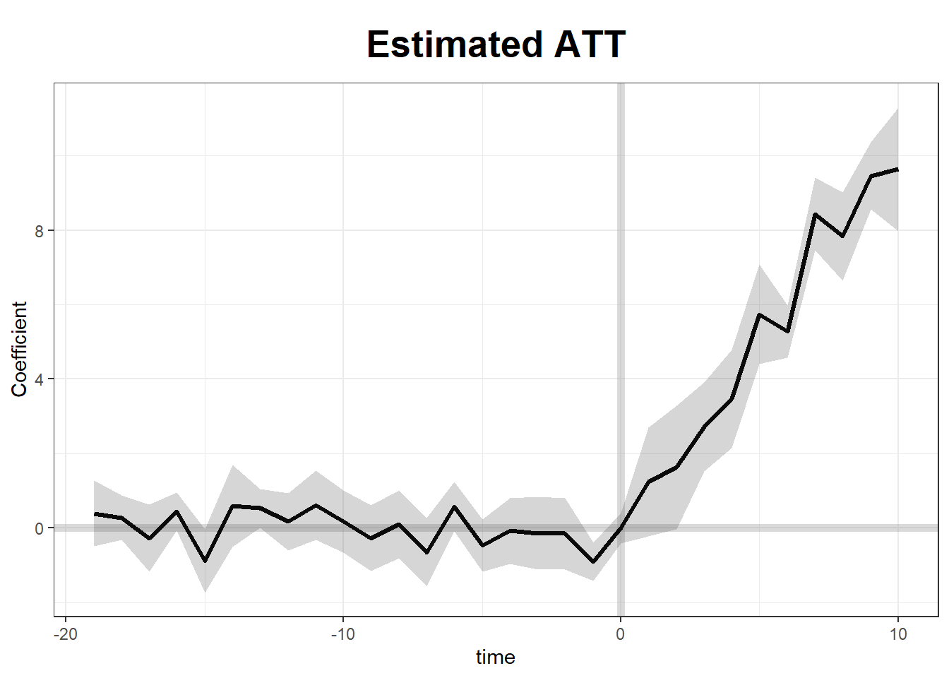

Figure 32.1: Generalized synthetic control fit on the bundled gsynth simdata, with two-way fixed effects, cross-validated factor count, and parametric bootstrap standard errors.

---

32.10 Bayesian Synthetic Control

The Bayesian Synthetic Control (BSC) approach introduces a probabilistic alternative to traditional synthetic control methods. Unlike the standard SCM, which estimates a single point estimate of treatment effects using a convex combination of control units, BSC incorporates posterior predictive distributions, allowing for proper uncertainty quantification and probabilistic inference​.

Bayesian methods offer several advantages over frequentist SCM:

• Probabilistic Treatment Effects: Instead of a single deterministic estimate, Bayesian SCM provides a distribution over possible treatment effects.

• Regularization via Priors: Bayesian approaches allow for the incorporation of shrinkage priors to improve estimation stability in high-dimensional settings.

• Flexibility: The Bayesian framework can accommodate dynamic latent factor models, addressing issues like time-varying heterogeneity​.

Two major Bayesian approaches to SCM:

1. Dynamic Multilevel Factor Models (Pang, Liu, and Xu 2022)
2. Bayesian Sparse Synthetic Control (S. Kim, Lee, and Gupta 2020)

32.10.1 Bayesian Causal Inference Framework

In the traditional SCM, we estimate the counterfactual outcome \(Y_{it}(0)\) for treated unit \(i\) at time \(t\) using a weighted sum of control units:

\[ \hat{Y}_{it}(0) = \sum_{j \neq i} w_j Y_{jt}. \]

However, this deterministic approach does not quantify uncertainty in the estimation. The Bayesian SCM instead models the counterfactual outcome as a posterior predictive distribution:

\[ P(Y_{it}(0) | Y_{\text{obs}}, \theta), \]

where \(\theta\) represents the parameters of the model (e.g., factor loadings, regression coefficients, latent variables). The Bayesian approach estimates full posterior distributions, allowing us to compute credible intervals instead of relying solely on point estimates.

32.10.2 Bayesian Dynamic Multilevel Factor Model

The Dynamic Multilevel Factor Model (DM-LFM), proposed by Pang, Liu, and Xu (2022), extends SCM by incorporating latent factor models to correct for unit-specific time trends.

32.10.2.1 Model Specification

Let \(Y_{it}\) be the observed outcome for unit \(i\) at time \(t\). The potential untreated outcome follows:

\[ Y_{it}(0) = X_{it} \beta + \lambda_i' f_t + \varepsilon_{it}, \]

where:

• \(X_{it}\) are observed covariates,

• \(\beta\) are regression coefficients,

• \(\lambda_i\) are unit-specific factor loadings,

• \(f_t\) are common latent time factors,

• \(\varepsilon_{it} \sim \mathcal{N}(0, \sigma^2)\) is the noise term.

The treatment effect is defined as:

\[ \tau_{it} = Y_{it}(1) - Y_{it}(0). \]

Under latent ignorability, we assume:

\[ P(T_i | X_i, U_i) = P(T_i | X_i), \]

where \(U_i\) are latent variables extracted from the outcome data​.

32.10.2.2 Bayesian Inference Procedure

To estimate treatment effects, we follow these steps:

1. Estimate \(\lambda_i\) and \(f_t\) using control units.
2. Predict counterfactuals for treated units: \[ \hat{Y}_{it}(0) = X_{it} \hat{\beta} + \hat{\lambda}_i' \hat{f}_t. \]
3. Obtain the posterior predictive distribution of treatment effects.

This Bayesian approach enables proper credible intervals for causal effects.

32.10.3 Bayesian Sparse Synthetic Control

S. Kim, Lee, and Gupta (2020) propose an alternative Bayesian framework that removes restrictive constraints imposed by standard SCM​.

32.10.3.1 Relaxing SCM Constraints

Traditional SCM imposes:

1. Nonnegative weights: \(w_j \geq 0\).
2. Convex combination: \(\sum_j w_j = 1\).

BSCM relaxes these by allowing negative weights and regularization priors. It models the control unit weights using Bayesian shrinkage priors:

\[ w_j \sim \mathcal{N}(0, \tau^2), \]

where \(\tau^2\) is a regularization parameter. This allows flexible weight selection while preventing overfitting.

32.10.3.2 Bayesian Shrinkage Priors

BSCM incorporates horseshoe priors and spike-and-slab priors to select relevant control units:

• Horseshoe Prior: \[ w_j \sim \mathcal{N}(0, \lambda_j^2), \quad \lambda_j \sim C^+(0,1). \]

• Spike-and-Slab Prior: \[ w_j \sim \gamma_j \mathcal{N}(0, \sigma_1^2) + (1-\gamma_j) \mathcal{N}(0, \sigma_0^2), \] where \(\gamma_j \sim \text{Bernoulli}(\pi)\) determines whether a control unit is included.

These priors ensure robust weight selection while controlling for overfitting.

32.10.4 Bayesian Inference and MCMC Estimation

Both DM-LFM and BSCM are estimated using Markov Chain Monte Carlo (MCMC). Given observed data \(Y_{\text{obs}}\), we sample from the posterior:

\[ P(\theta | Y_{\text{obs}}) \propto P(Y_{\text{obs}} | \theta) P(\theta), \]

where \(P(\theta)\) encodes prior beliefs about the parameters.

Common MCMC techniques used:

• Gibbs Sampling for latent factors and regression coefficients.

• Hamiltonian Monte Carlo (HMC) for high-dimensional posteriors.

Build note: the Bayesian SCM example below uses rstan, which requires a working C++ toolchain. On Windows install Rtools; on macOS install the Xcode command-line tools. First-time compilation can take 5-10 minutes. The chunk is set to eval = FALSE for exactly this reason, run it manually if you want to reproduce the output.

# Load necessary libraries
library(rstan)
library(bayesplot)

# Define Bayesian SCM model in Stan
scm_model <- "
data {
  int<lower=0> N;  // Number of observations
  int<lower=0> T;  // Time periods
  matrix[N, T] Y;  // Outcome matrix
}
parameters {
  vector[T] f;  // Latent factors
  vector[N] lambda; // Factor loadings
  real<lower=0> sigma; // Noise variance
}
model {
  // Priors
  f ~ normal(0, 1);
  lambda ~ normal(0, 1);

  // Likelihood
  for (i in 1:N)
    Y[i, ] ~ normal(lambda[i] * f, sigma);
}
"

# Compile and fit the model
fit <-
  stan(model_code = scm_model, data = list(
    N = 50,
    T = 20,
    Y = matrix(rnorm(1000), 50, 20)
  ))

# Summarize results
print(fit)

32.11 Using Multiple Outcomes to Improve the Synthetic Control Method

Typically, SCM constructs a weighted combination of untreated control units to approximate the counterfactual outcome of the treated unit. However, standard SCM is limited to a single outcome variable, which can lead to biased estimates when multiple correlated outcomes are available.

In their work, L. Sun, Ben-Michael, and Feller (2025) propose a novel extension of SCM that leverages multiple outcome variables to improve causal inference by:

1. Using a common set of synthetic control weights across all outcomes rather than estimating separate weights for each outcome.
2. Reducing bias using a low-rank factor model, which exploits shared latent structures across outcomes.

32.11.1 Standard Synthetic Control Method

Let \(Y_{itk}\) denote the observed outcome for unit \(i\) at time \(t\) for outcome \(k\), where \(i = 1, \dots, N\), \(t = 1, \dots, T\), and \(k = 1, \dots, K\). The potential outcomes framework assumes:

\[ Y_{itk}(d) = \mu_{itk} + \delta_{itk} d + \varepsilon_{itk}, \quad d \in {0,1} \]

where:

• \(\mu_{itk}\) represents the latent structure of untreated outcomes.

• \(\delta_{itk}\) is the treatment effect.

• \(\varepsilon_{itk} \sim \mathcal{N}(0, \sigma^2)\) is random noise.

For unit \(i=1\) (the treated unit), the observed outcome follows:

\[ Y_{1tk} = Y_{1tk}(0) + D_{1t} \delta_{1tk} \]

where \(D_{1t}\) is an indicator for treatment at time \(t\). The challenge is to estimate the counterfactual outcome \(Y_{1tk}(0)\), which is unobserved post-treatment.

SCM estimates \(Y_{1tk}(0)\) as a weighted combination of control units:

\[ \hat{Y}_{1tk}(0) = \sum_{i=2}^{N} w_i Y_{itk} \]

where weights \(w_i\) are chosen to minimize pre-treatment imbalance.

32.11.2 Using Multiple Outcomes for Bias Reduction

Instead of estimating separate weights \(w_k\) for each outcome \(k\), L. Sun, Ben-Michael, and Feller (2025) propose a single set of weights \(w\) across all outcomes. This approach is justified under a low-rank factor model, which assumes that multiple outcomes share common latent factors.

32.11.2.1 Low-Rank Factor Model

Assume the untreated potential outcome follows a linear factor structure:

\[ Y_{itk}(0) = X_{it} \beta_k + \lambda_i' f_{tk} + \varepsilon_{itk} \]

where:

• \(X_{it}\) are observed covariates.

• \(\beta_k\) are outcome-specific coefficients.

• \(\lambda_i\) are unit-specific factor loadings.

• \(f_{tk}\) are time-and-outcome-specific latent factors.

If all outcomes share the same latent factor structure, then the bias in synthetic control estimation can be reduced by a factor of \(1 / \sqrt{K}\) as the number of outcomes \(K\) increases.

32.11.3 Estimation Methods

L. Sun, Ben-Michael, and Feller (2025) propose two methods for constructing a common synthetic control:

1. Concatenated Outcome Weights: Estimate weights by minimizing imbalance across all outcomes simultaneously:

   \[ \hat{w} = \arg\min_w \sum_{k=1}^{K} || Y_{1,\text{pre},k} - \sum_{i=2}^{N} w_i Y_{i,\text{pre},k} ||^2 \]

2. Averaged Outcome Weights: Estimate weights based on a linear combination (e.g., average) of outcomes:

   \[ \hat{w} = \arg\min_w || \frac{1}{K} \sum_{k=1}^{K} Y_{1,\text{pre},k} - \sum_{i=2}^{N} w_i \frac{1}{K} \sum_{k=1}^{K} Y_{i,\text{pre},k} ||^2 \]

These methods improve SCM performance by reducing variance and overfitting to noise.

32.11.4 Empirical Application: Flint Water Crisis

To illustrate the benefits of multiple outcome SCM, L. Sun, Ben-Michael, and Feller (2025) re-analyze the Flint water crisis, which led to lead contamination in drinking water, potentially affecting student performance.

Four key educational outcomes were studied:

1. Math Achievement
2. Reading Achievement
3. Special Needs Status
4. Daily Attendance

By applying common weights across these outcomes, their SCM results showed:

• Reduced bias and improved robustness compared to separate SCM fits.

• Better pre-treatment fit for educational outcomes.

• Stronger evidence of educational impacts following the crisis.

# Load necessary libraries
library(augsynth)

# Fit SCM using a common set of weights across multiple outcomes
synth_model <- augsynth_multiout()

---

32.12 Applications

32.12.1 Synthetic Control Estimation

This example simulates data for 10 states over 30 years, where State A receives treatment after year 15. We implement two approaches:

1. Standard Synthetic Control using Synth.
2. Generalized Synthetic Control using gsynth, which incorporates iterative fixed effects and multiple treated units.

Load Required Libraries

# install.packages("Synth")
# install.packages("gsynth")
library("Synth")
library("gsynth")

We construct a panel dataset where the outcome variable \(Y\) is influenced by two covariates (\(X_1, X_2\)). Treatment (\(T\)) is applied to State A from year 15 onwards, with an artificial treatment effect of +20.

# Simulate panel data
set.seed(1)

df <- data.frame(
  year      = rep(1:30, 10),          # 30 years for 10 states
  state     = rep(LETTERS[1:10], each = 30),  # States A to J
  X1        = round(rnorm(300, 2, 1), 2),     # Continuous covariate
  X2        = round(rbinom(300, 1, 0.5) + rnorm(300), 2),  # Binary + noise
  state.num = rep(1:10, each = 30)    # Numeric identifier for states
)

# Outcome variable: Y = 1 + 2 * X1 + noise
df$Y <- round(1 + 2 * df$X1 + rnorm(300), 2)

# Assign treatment: Only State A (state == "A") from year 15 onward
df$T <- as.integer(df$state == "A" & df$year >= 15)

# Apply treatment effect: Increase Y by 20 where treatment is applied
df$Y[df$T == 1] <- df$Y[df$T == 1] + 20

# View data structure
str(df)
#> 'data.frame':    300 obs. of  7 variables:
#>  $ year     : int  1 2 3 4 5 6 7 8 9 10 ...
#>  $ state    : chr  "A" "A" "A" "A" ...
#>  $ X1       : num  1.37 2.18 1.16 3.6 2.33 1.18 2.49 2.74 2.58 1.69 ...
#>  $ X2       : num  1.96 0.4 -0.75 -0.56 -0.45 1.06 0.51 -2.1 0 0.54 ...
#>  $ state.num: int  1 1 1 1 1 1 1 1 1 1 ...
#>  $ Y        : num  2.29 4.51 2.07 8.87 4.37 1.32 8 7.49 6.98 3.72 ...
#>  $ T        : int  0 0 0 0 0 0 0 0 0 0 ...

32.12.1.1 Step 1: Estimating Synthetic Control with Synth

The Synth package creates a synthetic control by matching pre-treatment trends of the treated unit (State A) with a weighted combination of donor states.

We specify predictors, dependent variable, and donor pool.

dataprep.out <- dataprep(
  df,
  predictors = c("X1", "X2"),
  dependent = "Y",
  unit.variable = "state.num",
  time.variable = "year",
  unit.names.variable = "state",
  treatment.identifier = 1,
  controls.identifier = 2:10,
  time.predictors.prior = 1:14,
  time.optimize.ssr = 1:14,
  time.plot = 1:30
)

Fit Synthetic Control Model

synth.out <- synth(dataprep.out)
#> 
#> X1, X0, Z1, Z0 all come directly from dataprep object.
#> 
#> 
#> **************** 
#>  searching for synthetic control unit  
#>  
#> 
#> **************** 
#> **************** 
#> **************** 
#> 
#> MSPE (LOSS V): 9.831789 
#> 
#> solution.v:
#>  0.3888387 0.6111613 
#> 
#> solution.w:
#>  0.1115941 0.1832781 0.1027237 0.312091 0.06096758 0.03509706 0.05893735 0.05746256 0.07784853

# Display synthetic control weights and balance table
print(synth.tab(dataprep.res = dataprep.out, synth.res = synth.out))
#> $tab.pred
#>    Treated Synthetic Sample Mean
#> X1   2.028     2.028       2.017
#> X2   0.513     0.513       0.394
#> 
#> $tab.v
#>    v.weights
#> X1 0.389    
#> X2 0.611    
#> 
#> $tab.w
#>    w.weights unit.names unit.numbers
#> 2      0.112          B            2
#> 3      0.183          C            3
#> 4      0.103          D            4
#> 5      0.312          E            5
#> 6      0.061          F            6
#> 7      0.035          G            7
#> 8      0.059          H            8
#> 9      0.057          I            9
#> 10     0.078          J           10
#> 
#> $tab.loss
#>            Loss W   Loss V
#> [1,] 9.761708e-12 9.831789

Plot: Observed vs. Synthetic State A. Figure 32.2 overlays the actual outcome trajectory of State A with its synthetic counterfactual.

path.plot(
  synth.out,
  dataprep.out,
  Ylab = "Y",
  Xlab = "Year",
  Legend = c("State A", "Synthetic State A"),
  Legend.position = "topleft"
)

# Mark the treatment start year
abline(v = 15, lty = 2)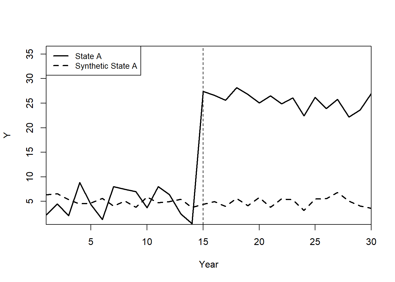

Figure 32.2: Path plot comparing the observed outcome of treated State A with its synthetic-control counterfactual; the dashed vertical line marks the treatment start at year 15.

Plot: Treatment Effect (Gaps Plot)

The gaps plot shows the difference between State A and its synthetic control over time. Figure 32.3 plots this treatment-effect path.

gaps.plot(synth.res    = synth.out,
          dataprep.res = dataprep.out,
          Ylab         = c("Gap"),
          Xlab         = c("Year"),
          Ylim         = c(-30, 30),
          Main         = ""
)

abline(v   = 15, lty = 2)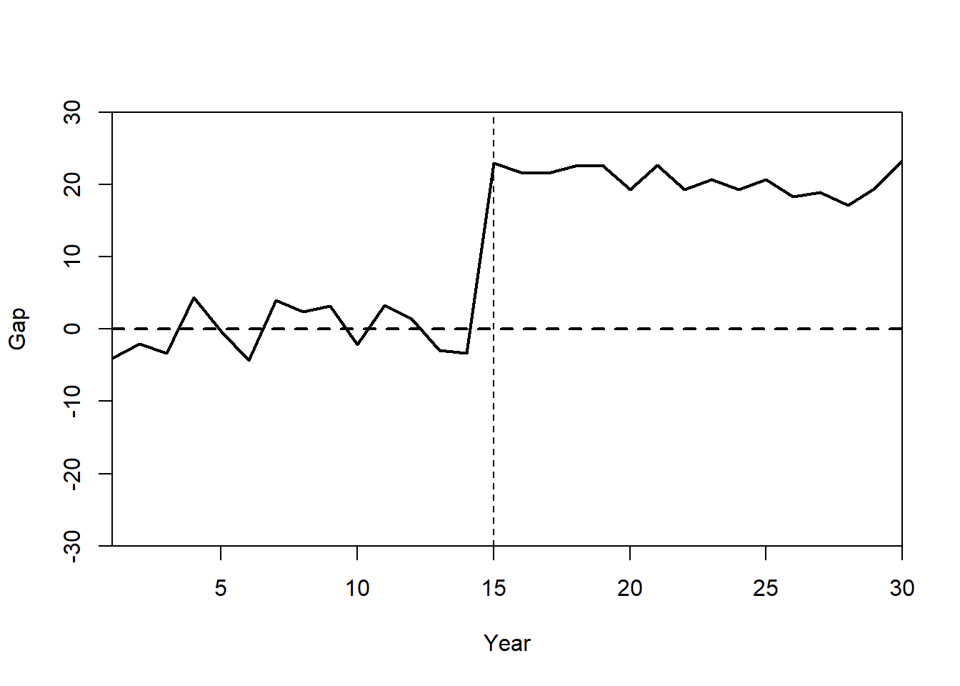

Figure 32.3: Gaps plot showing the period-by-period difference between the observed outcome of State A and its synthetic counterfactual; the post-1975 deviation indicates the estimated treatment effect.

32.12.1.2 Modern alternatives: tidysynth and augsynth

The classic Synth workflow above relies on building a dataprep matrix of predictors, treated/donor identifiers, and time windows before invoking synth(). Two more recent packages streamline this pipeline:

• tidysynth (Dunford) provides a tidyverse-style API in which the synthetic-control workflow is expressed as a chained sequence of verbs, synthetic_control() initializes the object, generate_predictor() defines pre-treatment matching variables, generate_weights() solves for donor weights, and generate_control() constructs the synthetic counterfactual. Diagnostics, plots, and placebo tests are dispatched on the resulting object via S3 methods (plot_trends(), plot_placebos(), grab_significance()), avoiding the matrix bookkeeping required by Synth::dataprep().
• augsynth (Ben-Michael, Feller, and Rothstein), already used elsewhere in this chapter (see Section Augmented Synthetic Control Method), implements ridge-augmented synthetic control with explicit bias correction and is the recommended package when pre-treatment fit is poor.

A minimal tidysynth skeleton, parallel to the Synth example above, is:

# install.packages("tidysynth")
library(tidysynth)
library(dplyr)

# `df` is a long-format panel with state, year, Y, X1, X2;
# state == "State A" is treated, intervention at year 15.
sc_out <- df %>%
    synthetic_control(
        outcome      = Y,
        unit         = state,
        time         = year,
        i_unit       = "State A",
        i_time       = 15,
        generate_placebos = TRUE
    ) %>%
    generate_predictor(
        time_window = 1:14,
        X1_mean     = mean(X1, na.rm = TRUE),
        X2_mean     = mean(X2, na.rm = TRUE)
    ) %>%
    generate_weights(
        optimization_window = 1:14,
        margin_ipop         = 0.02,
        sigf_ipop           = 7,
        bound_ipop          = 6
    ) %>%
    generate_control()

sc_out %>% plot_trends()
sc_out %>% plot_placebos()
sc_out %>% grab_significance()
# See https://github.com/edunford/tidysynth for full examples.

The conceptual model is identical to Synth, a convex combination of donor units that minimizes pre-treatment outcome (and predictor) discrepancies, but the chained pipeline keeps the data, weights, and synthetic counterfactual bound to a single tibble-like object, which is convenient for embedding inside dplyr/purrr workflows and for batch placebo inference.

---

32.12.1.3 Step 2: Estimating Generalized Synthetic Control with gsynth

Unlike Synth, the gsynth package supports:

• Iterative Fixed Effects (IFE) for unobserved heterogeneity.

• Multiple Treated Units and Staggered Adoption.

• Bootstrapped Standard Errors for inference.

Fit Generalized Synthetic Control Model

We use two-way fixed effects, cross-validation (CV = TRUE), and bootstrapped standard errors.

gsynth.out <- gsynth(
  Y ~ T + X1 + X2,
  data = df,
  index = c("state", "year"),
  force = "two-way",
  CV = TRUE,
  r = c(0, 5),
  se = TRUE,
  inference = "parametric",
  nboots = 100
)
#> Parallel computing ...
#> Cross-validating ... 
#>  r = 0; sigma2 = 1.13533; IC = 0.95632; PC = 0.96713; MSPE = 1.65502
#>  r = 1; sigma2 = 0.96885; IC = 1.54420; PC = 4.30644; MSPE = 1.33375
#>  r = 2; sigma2 = 0.81855; IC = 2.08062; PC = 6.58556; MSPE = 1.27341*
#>  r = 3; sigma2 = 0.71670; IC = 2.61125; PC = 8.35187; MSPE = 1.79319
#>  r = 4; sigma2 = 0.62823; IC = 3.10156; PC = 9.59221; MSPE = 2.02301
#>  r = 5; sigma2 = 0.55497; IC = 3.55814; PC = 10.48406; MSPE = 2.79596
#> 
#>  r* = 2
#> 
#> 
Simulating errors ...
Bootstrapping ...
#> 

Figure ?? renders the GSC treatment-effect, counterfactual, and control-case panels for the simulated State A example.

# Plot Estimated Treatment Effects
plot(gsynth.out)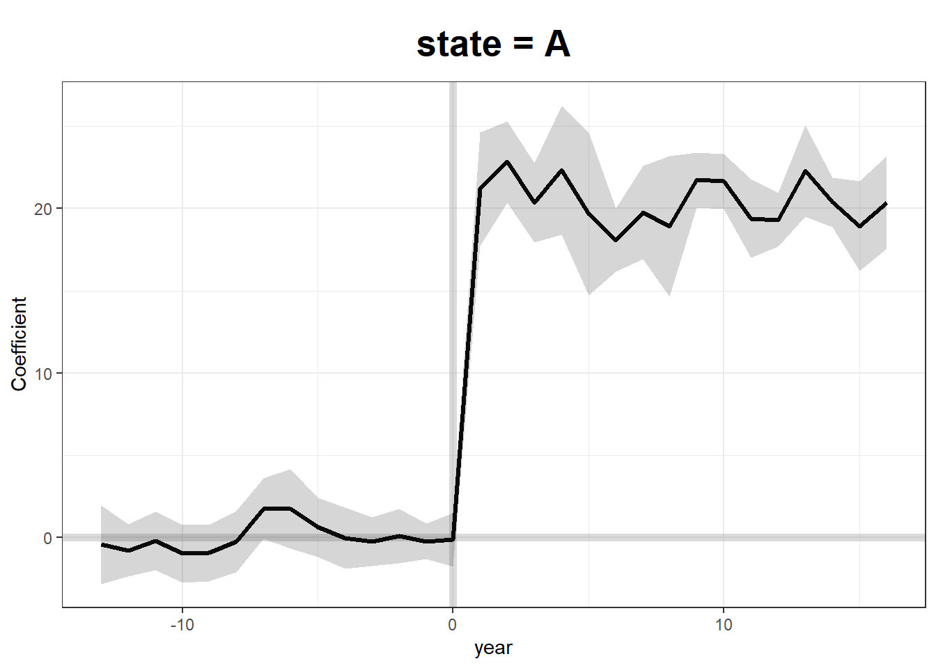

Figure 32.4: Generalized synthetic control output for the simulated State A example, showing estimated treatment effects, the counterfactual trajectory, and the raw control-unit trajectories.

# Plot Counterfactual Trends
plot(gsynth.out, type = "counterfactual")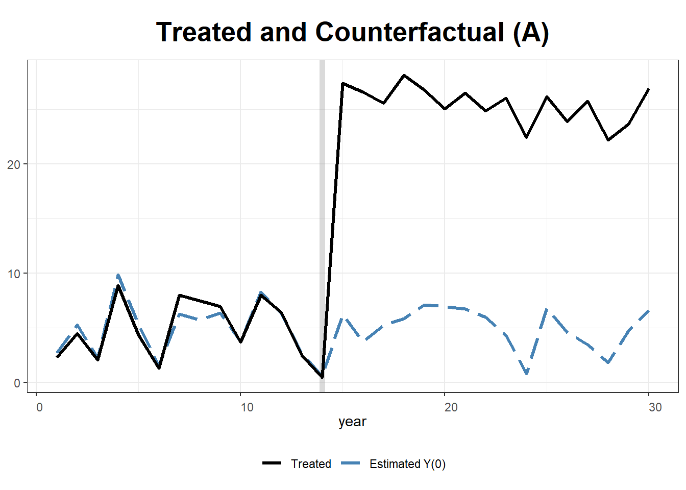

Figure 32.5: Generalized synthetic control output for the simulated State A example, showing estimated treatment effects, the counterfactual trajectory, and the raw control-unit trajectories.

# Show Estimations for Control Cases
plot(gsynth.out, type = "counterfactual", raw = "all")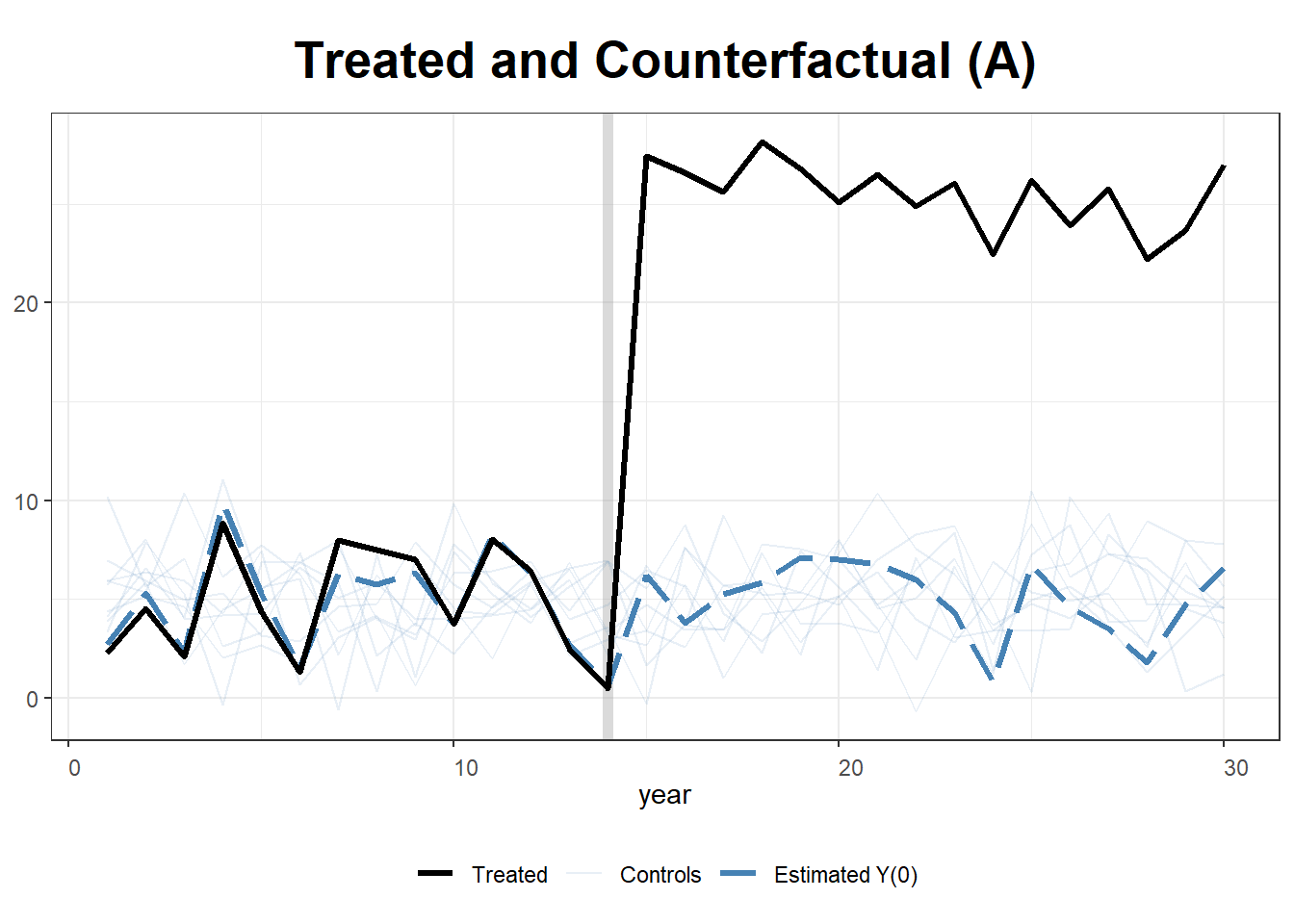

Figure 32.6: Generalized synthetic control output for the simulated State A example, showing estimated treatment effects, the counterfactual trajectory, and the raw control-unit trajectories.

32.12.2 The Basque Country Policy Change

The Basque Country in Spain implemented a major policy change in 1975, impacting its GDP per capita growth. This example uses SCM to estimate the counterfactual economic performance had the policy not been implemented.

We will:

1. Construct a synthetic control using economic predictors.
2. Evaluate the policy’s impact by comparing the real and synthetic Basque GDP.

library(Synth)

The basque dataset from Synth contains economic indicators for Spain’s regions from 1955 to 1997.

data("basque")
dim(basque)  # 774 observations, 17 variables
#> [1] 774  17
head(basque)
#>   regionno     regionname year   gdpcap sec.agriculture sec.energy sec.industry
#> 1        1 Spain (Espana) 1955 2.354542              NA         NA           NA
#> 2        1 Spain (Espana) 1956 2.480149              NA         NA           NA
#> 3        1 Spain (Espana) 1957 2.603613              NA         NA           NA
#> 4        1 Spain (Espana) 1958 2.637104              NA         NA           NA
#> 5        1 Spain (Espana) 1959 2.669880              NA         NA           NA
#> 6        1 Spain (Espana) 1960 2.869966              NA         NA           NA
#>   sec.construction sec.services.venta sec.services.nonventa school.illit
#> 1               NA                 NA                    NA           NA
#> 2               NA                 NA                    NA           NA
#> 3               NA                 NA                    NA           NA
#> 4               NA                 NA                    NA           NA
#> 5               NA                 NA                    NA           NA
#> 6               NA                 NA                    NA           NA
#>   school.prim school.med school.high school.post.high popdens invest
#> 1          NA         NA          NA               NA      NA     NA
#> 2          NA         NA          NA               NA      NA     NA
#> 3          NA         NA          NA               NA      NA     NA
#> 4          NA         NA          NA               NA      NA     NA
#> 5          NA         NA          NA               NA      NA     NA
#> 6          NA         NA          NA               NA      NA     NA

32.12.2.1 Step 1: Preparing Data for Synth

We define predictors and specify pre-treatment (1960–1969) and post-treatment (1975–1997) periods.

dataprep.out <- dataprep(
    foo = basque,
    predictors = c(
        "school.illit",
        "school.prim",
        "school.med",
        "school.high",
        "school.post.high",
        "invest"
    ),
    predictors.op = "mean",
    time.predictors.prior = 1964:1969,
    # Pre-treatment period
    special.predictors = list(
        list("gdpcap", 1960:1969, "mean"),
        list("sec.agriculture", seq(1961, 1969, 2), "mean"),
        list("sec.energy", seq(1961, 1969, 2), "mean"),
        list("sec.industry", seq(1961, 1969, 2), "mean"),
        list("sec.construction", seq(1961, 1969, 2), "mean"),
        list("sec.services.venta", seq(1961, 1969, 2), "mean"),
        list("sec.services.nonventa", seq(1961, 1969, 2), "mean"),
        list("popdens", 1969, "mean")
    ),
    dependent = "gdpcap",
    unit.variable = "regionno",
    unit.names.variable = "regionname",
    time.variable = "year",
    treatment.identifier = 17,
    # Basque region
    controls.identifier = c(2:16, 18),
    # Control regions
    time.optimize.ssr = 1960:1969,
    time.plot = 1955:1997
)

32.12.2.2 Step 2: Estimating the Synthetic Control

We now estimate the synthetic control weights using synth(). This solves for weights that best match the pre-treatment economic indicators of the Basque Country.

synth.out = synth(data.prep.obj = dataprep.out, method = "BFGS")
#> 
#> X1, X0, Z1, Z0 all come directly from dataprep object.
#> 
#> 
#> **************** 
#>  searching for synthetic control unit  
#>  
#> 
#> **************** 
#> **************** 
#> **************** 
#> 
#> MSPE (LOSS V): 0.008864606 
#> 
#> solution.v:
#>  0.02773094 1.194e-07 1.60609e-05 0.0007163836 1.486e-07 0.002423908 0.0587055 0.2651997 0.02851006 0.291276 0.007994382 0.004053188 0.009398579 0.303975 
#> 
#> solution.w:
#>  2.53e-08 4.63e-08 6.44e-08 2.81e-08 3.37e-08 4.844e-07 4.2e-08 4.69e-08 0.8508145 9.75e-08 3.2e-08 5.54e-08 0.1491843 4.86e-08 9.89e-08 1.162e-07

32.12.2.3 Step 3: Evaluating Treatment Effects

Calculate the GDP Gap Between Real and Synthetic Basque Country

gaps = dataprep.out$Y1plot - (dataprep.out$Y0plot %*% synth.out$solution.w)
gaps[1:3,1]  # First three differences
#>       1955       1956       1957 
#> 0.15023473 0.09168035 0.03716475

The synth.tab() function provides pre-treatment fit diagnostics and predictor weights.

synth.tables = synth.tab(dataprep.res = dataprep.out, synth.res = synth.out)
names(synth.tables)
#> [1] "tab.pred" "tab.v"    "tab.w"    "tab.loss"

# Predictor Balance Table
synth.tables$tab.pred[1:13,]
#>                                          Treated Synthetic Sample Mean
#> school.illit                              39.888   256.337     170.786
#> school.prim                             1031.742  2730.104    1127.186
#> school.med                                90.359   223.340      76.260
#> school.high                               25.728    63.437      24.235
#> school.post.high                          13.480    36.153      13.478
#> invest                                    24.647    21.583      21.424
#> special.gdpcap.1960.1969                   5.285     5.271       3.581
#> special.sec.agriculture.1961.1969          6.844     6.179      21.353
#> special.sec.energy.1961.1969               4.106     2.760       5.310
#> special.sec.industry.1961.1969            45.082    37.636      22.425
#> special.sec.construction.1961.1969         6.150     6.952       7.276
#> special.sec.services.venta.1961.1969      33.754    41.104      36.528
#> special.sec.services.nonventa.1961.1969    4.072     5.371       7.111

Importance of Each Control Region in the Synthetic Basque Country

synth.tables$tab.w[8:14, ]
#>    w.weights            unit.names unit.numbers
#> 9      0.000    Castilla-La Mancha            9
#> 10     0.851              Cataluna           10
#> 11     0.000  Comunidad Valenciana           11
#> 12     0.000           Extremadura           12
#> 13     0.000               Galicia           13
#> 14     0.149 Madrid (Comunidad De)           14
#> 15     0.000    Murcia (Region de)           15

32.12.2.4 Step 4: Visualizing Results

Plot Real vs. Synthetic GDP Per Capita. Figure 32.7 overlays the actual Basque GDP trajectory with its synthetic counterfactual.

path.plot(
    synth.res = synth.out,
    dataprep.res = dataprep.out,
    Ylab = "Real Per-Capita GDP (1986 USD, thousand)",
    Xlab = "Year",
    Ylim = c(0, 12),
    Legend = c("Basque Country", "Synthetic Basque Country"),
    Legend.position = "bottomright"
)

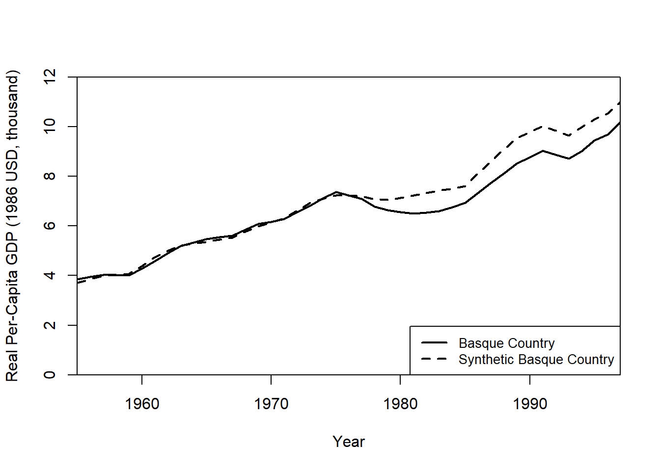
Figure 32.7: Path plot comparing real per-capita GDP for the Basque Country with its synthetic counterfactual constructed from a weighted combination of donor Spanish regions, 1955 to 1997.

Plot the Treatment Effect (GDP Gap). Figure 32.8 plots the period-by-period gap between actual and synthetic Basque GDP.

gaps.plot(
    synth.res = synth.out,
    dataprep.res = dataprep.out,
    Ylab = "Gap in Real Per-Capita GDP (1986 USD, thousand)",
    Xlab = "Year",
    Ylim = c(-1.5, 1.5),
    Main = NA
)

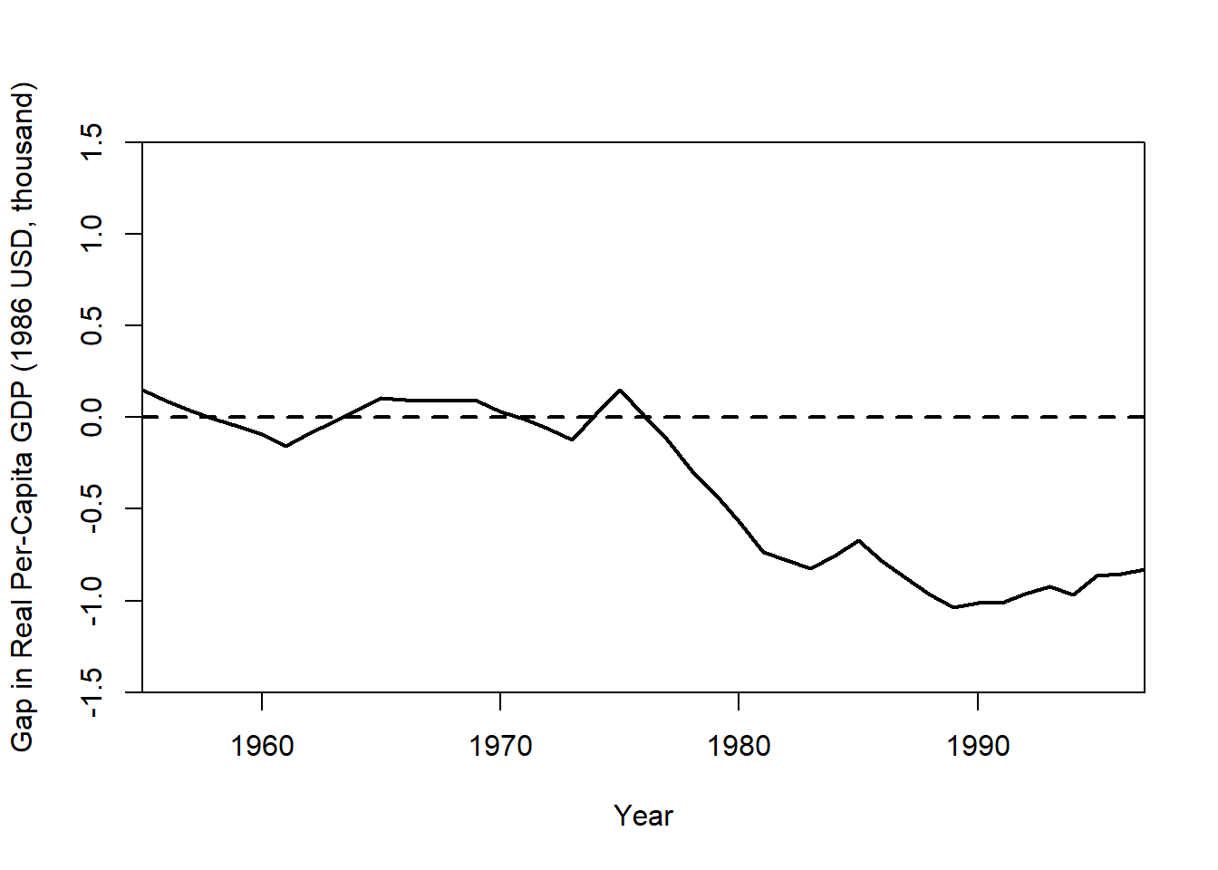
Figure 32.8: Gaps plot showing the difference between actual Basque per-capita GDP and its synthetic counterfactual; the large post-1975 deviation indicates the estimated impact of the policy change.

The gap plot shows the difference between actual Basque GDP and its synthetic control over time. A large post-treatment deviation suggests a policy impact.

32.12.3 Micro-Synthetic Control with microsynth

The microsynth package extends standard SCM by allowing:

1. Matching on both predictors and time-variant outcomes.
2. Permutation tests and jackknife resampling for placebo tests.
3. Multiple follow-up periods to track long-term treatment effects.
4. Omnibus test statistics for multiple outcome variables.

This example evaluates the Seattle Drug Market Initiative, a policing intervention aimed at reducing drug-related crime. The dataset seattledmi contains crime statistics across different city zones.

---

32.12.3.1 Step 1: Load the Required Package and Data

library(microsynth)
data("seattledmi")

32.12.3.2 Step 2: Define Predictors and Outcome Variables

We specify:

• Predictors (time-invariant): Population, race distribution, household data.

• Outcomes (time-variant): Crime rates across different offense categories.

cov.var <- c(
    "TotalPop",
    "BLACK",
    "HISPANIC",
    "Males_1521",
    "HOUSEHOLDS",
    "FAMILYHOUS",
    "FEMALE_HOU",
    "RENTER_HOU",
    "VACANT_HOU"
)
match.out <- c("i_felony", "i_misdemea", "i_drugs", "any_crime")

32.12.3.3 Step 3: Fit the Micro-Synthetic Control Model

We first estimate treatment effects using a single follow-up period.

sea1 <- microsynth(
    seattledmi,
    idvar       = "ID",          # Unique unit identifier
    timevar     = "time",        # Time variable
    intvar      = "Intervention",# Treatment assignment
    start.pre   = 1,             # Start of pre-treatment period
    end.pre     = 12,            # End of pre-treatment period
    end.post    = 16,            # End of post-treatment period
    match.out   = match.out,     # Outcomes to match on
    match.covar = cov.var,       # Predictors to match on
    result.var  = match.out,     # Variables for treatment effect estimates
    omnibus.var = match.out,     # Variables for omnibus p-values
    test        = "lower",       # One-sided test (decrease in crime)
    n.cores     = min(parallel::detectCores() - 4, 2) # Parallel processing
)

32.12.3.4 Step 4: Summarize Results

summary(sea1)

This output provides:

• Weighted unit contributions to the synthetic control.

• Treatment effect estimates and confidence intervals.

• p-values from permutation tests.

32.12.3.5 Step 5: Visualize the Treatment Effect

We generate a treatment effect plot comparing actual vs. synthetic trends.

plot_microsynth(sea1)

32.12.3.6 Step 6: Incorporating Multiple Follow-Up Periods

We extend the analysis by adding multiple post-treatment periods (end.post = c(14, 16)) and permutation-based placebo tests (perm = 250, jack = TRUE).

sea2 <- microsynth(
    seattledmi,
    idvar       = "ID",
    timevar     = "time",
    intvar      = "Intervention",
    start.pre   = 1,
    end.pre     = 12,
    end.post    = c(14, 16), # Two follow-up periods
    match.out   = match.out,
    match.covar = cov.var,
    result.var  = match.out,
    omnibus.var = match.out,
    test        = "lower",
    perm        = 250, # Permutation placebo tests
    jack        = TRUE, # Jackknife resampling
    n.cores     = min(parallel::detectCores() - 4, 2)
)

32.12.3.7 Step 7: Placebo Testing and Robustness Checks

Permutation and jackknife tests assess whether observed treatment effects are statistically significant or due to random fluctuations.

Key robustness checks:

1. Permutation Tests (perm = 250)
   • Reassigns treatment randomly and estimates placebo effects.
   • If true effects exceed placebo effects, they are likely causal.
2. Jackknife Resampling (jack = TRUE)
   • Removes one control unit at a time and re-estimates effects.
   • Ensures no single control dominates the synthetic match.

summary(sea2)  # Compare estimates with multiple follow-up periods
plot_microsynth(sea2)  # Visualize placebo-adjusted treatment effects

📖 Free preview — limited per publisher guidelines. Purchase the complete A Guide on Data Analysis series (Vols. 1–4) on Springer.

Vol. 1 Vol. 2 Vol. 3 Vol. 4