26 Decomposition Methods
The previous two chapters decompose a causal effect into the parts that travel through different channels. This chapter decomposes a difference: a wage gap between two groups, a change in an outcome between two periods, a coefficient that moves when controls are added, a variance that splits across sources. The two enterprises share arithmetic and almost nothing else, and conflating them is the most common error in the applied use of these tools.
The distinction is worth stating up front. A mediation decomposition asks what a treatment does on its way to an outcome, and every term in it is a contrast of potential outcomes. A Kitagawa-Oaxaca-Blinder decomposition asks how much of an observed gap between two groups would remain if the groups had the same characteristics, and its terms are contrasts of observed conditional means under a hypothetical reweighting. The second is a description of the data, and it becomes causal only under assumptions that the arithmetic itself never supplies (Fortin et al. 2011).
That said, decomposition is where a great deal of real mechanism evidence lives. When an applied paper reports that a coefficient falls by forty percent once industry controls are added, and concludes that industry composition explains forty percent of the effect, it is doing a decomposition badly. Doing it properly is the subject of Section 26.2, and it is probably the single most useful tool in this chapter for economists, finance researchers, and expert witnesses.
The chapter covers the aggregate mean decomposition and its identification problems, the conditional decomposition of covariate contributions, distributional decompositions that go beyond the mean, Shapley methods that resolve the ordering ambiguity that afflicts all of them, and variance decompositions in two-way fixed-effects models.
26.1 The Kitagawa-Oaxaca-Blinder Decomposition
The foundational device is due to Kitagawa (1955) in demography and independently to Oaxaca (1973) and Blinder (1973) in labor economics. Two groups, \(A\) and \(B\), differ in mean outcome. Fit a separate linear model in each group,
\[ Y_g = X_g' \beta_g + \varepsilon_g, \qquad g \in \{A, B\}, \]
so that \(\bar Y_g = \bar X_g' \hat\beta_g\) by the properties of least squares. The raw gap then splits as
\[ \bar Y_A - \bar Y_B = \underbrace{(\bar X_A - \bar X_B)' \hat\beta_B}_{\text{endowments}} \;+\; \underbrace{\bar X_B' (\hat\beta_A - \hat\beta_B)}_{\text{coefficients}} \;+\; \underbrace{(\bar X_A - \bar X_B)'(\hat\beta_A - \hat\beta_B)}_{\text{interaction}} . \]
This is the three-fold decomposition. The endowments term is what the gap would be if group \(B\)’s returns applied to the difference in characteristics; the coefficients term is what it would be if the two groups had group \(B\)’s characteristics but their own returns; the interaction term collects the remainder.
The two-fold version splits the gap into an explained part, attributable to differences in characteristics, and an unexplained part, attributable to everything else:
\[ \bar Y_A - \bar Y_B = \underbrace{(\bar X_A - \bar X_B)' \beta^*}_{\text{explained}} \;+\; \underbrace{\bar X_A'(\hat\beta_A - \beta^*) + \bar X_B'(\beta^* - \hat\beta_B)}_{\text{unexplained}}, \]
where \(\beta^*\) is a reference coefficient vector representing the returns that would prevail in the absence of the group difference. The choice of \(\beta^*\) is not determined by the data, and it matters a great deal.
26.1.1 Replication: The Chicago Nativity Wage Gap
The oaxaca package ships a sample of the 2000 Census public-use microdata for the Chicago metropolitan area, with log real hourly wage, nativity, sex, age, and education. The gap of interest is between native-born and foreign-born workers.
library(oaxaca)
data("chicago", package = "oaxaca")

ch   <- chicago[complete.cases(chicago), ]
covs <- c("age", "female", "LTHS", "some.college", "college", "advanced.degree")

gap <- mean(ch$ln.real.wage[ch$foreign.born == 0]) -
       mean(ch$ln.real.wage[ch$foreign.born == 1])

c(n = nrow(ch), share_foreign_born = mean(ch$foreign.born),
  log_wage_gap = gap)
#>                  n share_foreign_born       log_wage_gap
#>        666.0000000          0.5690691          0.1433657
Native-born workers earn about fourteen log points more. The decomposition asks how much of that survives once age, sex, and education are equalized.
fA <- lm(reformulate(covs, "ln.real.wage"), data = subset(ch, foreign.born == 0))
fB <- lm(reformulate(covs, "ln.real.wage"), data = subset(ch, foreign.born == 1))
fP <- lm(reformulate(covs, "ln.real.wage"), data = ch)   # pooled reference

xA <- colMeans(model.matrix(fA)); bA <- coef(fA)
xB <- colMeans(model.matrix(fB)); bB <- coef(fB)
bP <- coef(fP)

threefold <- c(
    endowments   = sum((xA - xB) * bB),
    coefficients = sum(xB * (bA - bB)),
    interaction  = sum((xA - xB) * (bA - bB))
)

explained <- sum((xA - xB) * bP)
twofold   <- c(explained = explained, unexplained = gap - explained)

round(c(threefold, sum = sum(threefold), twofold, raw_gap = gap), 4)
#>   endowments coefficients  interaction          sum    explained  unexplained
#>       0.0769       0.1222      -0.0558       0.1434       0.0683       0.0751
#>      raw_gap
#>       0.1434
Cross-checking against the package confirms the arithmetic and supplies bootstrap standard errors.
set.seed(1)
ox <- oaxaca(ln.real.wage ~ age + female + LTHS + some.college + college +
                 advanced.degree | foreign.born, data = ch, R = 200)
round(ox$threefold$overall, 4)
#>   coef(endowments)     se(endowments) coef(coefficients)   se(coefficients)
#>             0.0769             0.0310             0.1222             0.0428
#>  coef(interaction)    se(interaction)
#>            -0.0558             0.0386
26.1.2 The Index Number Problem
The two-fold decomposition needs a reference coefficient vector, and the literature offers at least half a dozen candidates: group \(A\)’s coefficients, group \(B\)’s coefficients, a simple average, a sample-share weighted average, the pooled regression with a group dummy (Neumark 1988), and the pooled regression without one (Oaxaca and Ransom 1994). Each corresponds to a different implicit counterfactual about which group’s returns are the “non-discriminatory” ones, and the data cannot choose among them.
How much does it matter?
refs <- list(`group A returns` = bA,
             `group B returns` = bB,
             `pooled`          = bP,
             `simple average`  = (bA + bB) / 2)

sens <- sapply(refs, function(b) {
    e <- sum((xA - xB) * b)
    c(explained = e, unexplained = gap - e, share_explained = e / gap)
})

knitr::kable(
    round(sens, 4),
    caption = paste("The same wage gap decomposed under four choices of",
                    "reference coefficient vector. The share of the gap",
                    "attributed to characteristics rather than to returns",
                    "varies by more than a factor of three, and nothing in",
                    "the data adjudicates the choice.")
)| group A returns | group B returns | pooled | simple average | |
|---|---|---|---|---|
| explained | 0.0211 | 0.0769 | 0.0683 | 0.0490 |
| unexplained | 0.1222 | 0.0664 | 0.0751 | 0.0943 |
| share_explained | 0.1474 | 0.5367 | 0.4761 | 0.3421 |
The explained share ranges from about fifteen percent to about fifty-four percent depending on a choice the analyst makes before seeing any results. Any decomposition reported without stating the reference vector, and ideally without showing this sensitivity table, is not reproducible in any meaningful sense.
26.1.3 The Detailed Decomposition Is Not Invariant
A second and more insidious identification problem afflicts the detailed decomposition, which attributes parts of the unexplained component to individual covariates. When the regressors include a set of dummy variables with an omitted reference category, the split of the unexplained component between the intercept and the individual dummies depends on which category was omitted (Oaxaca and Ransom 1999). Changing the base education category changes the reported contribution of education to discrimination, with no change to the total.
Yun (2005) gives the standard fix: normalize the dummy coefficients so that they sum to zero within each categorical variable, which makes the intercept the grand mean rather than the omitted category’s value and renders the detailed decomposition invariant to the base. This normalization is not the default in most software, and detailed decompositions of categorical variables reported without it should be treated as arbitrary.
A related warning applies to the linear specification itself. Barsky et al. (2002) show, in the context of the Black-White wealth gap, that when the covariate distributions of the two groups overlap poorly, the linear decomposition extrapolates heavily and can be badly wrong; they propose a nonparametric reweighting alternative. Ñopo (2008) makes the common-support problem explicit by decomposing the gap into four parts, one of which is attributable to the region of covariate space where one group has no counterpart in the other. Reporting the fraction of each group that lies outside the other’s common support is a minimum diagnostic.
26.1.4 When Is a Decomposition Causal?
The explained component has a causal interpretation only under conditions that are stronger than they look (Fortin et al. 2011). Ignorability requires that group membership be as good as randomly assigned conditional on the covariates, which for immutable characteristics is a strange thing to assert. Overlap requires common support. And the counterfactual must be a well-defined intervention: “what if foreign-born workers had native-born workers’ education” presupposes an intervention on education that leaves everything else fixed.
VanderWeele and Robinson (2014) make the point for the specific and consequential case of race in regression models. Adjusting for a mediator of the race effect, such as education, yields a controlled direct effect of race holding education fixed, which is not “the effect of discrimination” and is often not any quantity of policy interest. Their recommended reframing, developed further in Jackson and VanderWeele (2018), is to ask about disparity reduction: how much would the gap fall under a specified intervention that changes the distribution of the mediator in the disadvantaged group to match the advantaged group’s? That estimand is well defined, it corresponds to something a policy could do, and it is estimated by the reweighting methods of Section 26.3 rather than by the coefficients term of an Oaxaca decomposition.
The safe reading of a Kitagawa-Oaxaca-Blinder decomposition is descriptive: this is how much of the gap is accounted for by differences in the listed characteristics, given the fitted models. The unexplained component is not “discrimination”; it is everything not in \(X\), including omitted variables, functional form error, and measurement error, and it grows mechanically as the covariate list shrinks.
26.2 The Conditional Decomposition of Covariate Contributions
Applied papers constantly report a sequence of specifications: the coefficient of interest is \(\beta\) with no controls, \(\beta'\) with demographic controls, \(\beta''\) with industry controls, and so on. The narrative attached to the shrinkage is a mechanism claim: “most of the raw gap is explained by industry sorting.”
This narrative has two defects. The attribution is order-dependent, so the contribution assigned to industry depends on whether industry was added second or fifth. And no standard error is attached, so a coefficient movement that is entirely sampling noise is reported as substantive.
Gelbach (2016) solves both problems, and the solution is elegant enough to derive in a paragraph. Let the base specification regress \(y\) on \(X_1\), and the full specification on \(X_1\) and \(X_2\). By the Frisch-Waugh-Lovell theorem, the omitted-variable-bias formula gives
\[ \hat\beta_1^{\text{base}} - \hat\beta_1^{\text{full}} = (X_1'X_1)^{-1} X_1' X_2 \, \hat\beta_2 = \hat\Gamma \hat\beta_2, \]
where the \(k\)-th column of \(\hat\Gamma\) holds the coefficients from regressing the \(k\)-th variable in \(X_2\) on \(X_1\). The total coefficient movement therefore decomposes exactly into one term per omitted covariate, \(\hat\Gamma_{\cdot k} \hat\beta_{2k}\), and the decomposition is invariant to the order in which the covariates are considered, because it never considers them in an order at all. Because both \(\hat\Gamma\) and \(\hat\beta_2\) are estimated by least squares, the delta method gives standard errors for each contribution.
base <- lm(ln.real.wage ~ foreign.born, data = ch)
full <- lm(reformulate(c("foreign.born", covs), "ln.real.wage"), data = ch)

X1  <- model.matrix(base)
X2  <- model.matrix(full)[, covs, drop = FALSE]
Gam <- solve(crossprod(X1), crossprod(X1, X2))    # auxiliary regressions
contrib <- Gam["foreign.born", ] * coef(full)[covs]

round(c(contrib,
        TOTAL          = sum(contrib),
        base_coef      = coef(base)[["foreign.born"]],
        full_coef      = coef(full)[["foreign.born"]],
        actual_change  = coef(base)[["foreign.born"]] -
                         coef(full)[["foreign.born"]]), 4)
#>             age          female            LTHS    some.college         college
#>          0.0591          0.0203         -0.0494         -0.0325         -0.0175
#> advanced.degree           TOTAL       base_coef       full_coef   actual_change
#>         -0.0300         -0.0500         -0.1434         -0.0934         -0.0500
The decomposition is exact: the contributions sum to the coefficient movement to machine precision. Substantively it says something the sequential narrative would have missed entirely. The foreign-born wage penalty falls from fourteen log points to nine when controls are added, a net movement of five log points, but that small net figure is the residue of two much larger offsetting forces. The four education terms together contribute about thirteen negative log points: foreign-born workers in this sample have less education, and equalizing education alone would close roughly ninety percent of the raw gap. Age pushes the other way by about six log points, because foreign-born workers are older and age is positively rewarded, so age was masking part of the penalty in the uncontrolled specification.
A sequential specification table would have shown the coefficient falling and invited the conclusion that controls “explain” the gap. The decomposition shows two large offsetting forces, one of which works against the story. This pattern, offsetting contributions that partially cancel in the total, is common and is invisible without the decomposition.
Two cautions. The decomposition is exact arithmetic about a specific pair of regressions; it inherits none of their causal credentials. And it answers “which covariates account for the coefficient movement”, not “which mechanisms carry the effect”. Reading it as mediation requires everything the mediation chapter requires, including the mediator-outcome unconfoundedness that a regression of this kind never delivers.
26.3 Distributional Decompositions
The mean is a poor summary of a gap that varies across the distribution. A wage gap may be near zero at the bottom, where minimum wages and institutional floors bind, and large at the top. Three families of methods extend decomposition beyond the mean.
26.3.1 Reweighting
DiNardo et al. (1996) introduced the workhorse. To construct the counterfactual distribution of group \(B\)’s outcomes under group \(A\)’s covariate distribution, reweight group \(B\) observations by
\[ \psi(x) = \frac{P(A \mid x)}{P(B \mid x)} \cdot \frac{P(B)}{P(A)}, \]
which is estimable from a single propensity model for group membership. The reweighted distribution answers “what would group \(B\)’s wage distribution look like if its members had group \(A\)’s characteristics but kept their own returns”, and comparing it to the two observed distributions splits any distributional statistic into a composition part and a structure part.
ps  <- glm(reformulate(covs, "foreign.born"), data = ch, family = binomial)
p   <- fitted(ps)
fb  <- ch$foreign.born == 1
pA  <- mean(!fb)

psi <- ((1 - p[fb]) / p[fb]) * ((1 - pA) / pA)   # DFL weights
psi <- psi / mean(psi)

mA  <- mean(ch$ln.real.wage[!fb])
mB  <- mean(ch$ln.real.wage[fb])
mCF <- weighted.mean(ch$ln.real.wage[fb], psi)

round(c(native = mA, foreign_born = mB, counterfactual = mCF,
        composition = mCF - mB, structure = mA - mCF,
        total = mA - mB), 4)
#>         native   foreign_born counterfactual    composition      structure
#>         2.6967         2.5534         2.6143         0.0609         0.0824
#>          total
#>         0.1434
The reweighting attributes about forty-two percent of the mean gap to composition and the rest to structure, which is close to the pooled-reference Oaxaca answer but obtained without imposing linearity on the outcome equation. That is the method’s main advantage: it requires a model for group membership rather than for the outcome, and the outcome enters only through weighted averages.
library(ggplot2)

dens <- rbind(
    data.frame(x = density(ch$ln.real.wage[!fb])$x,
               y = density(ch$ln.real.wage[!fb])$y, grp = "Native born"),
    data.frame(x = density(ch$ln.real.wage[fb])$x,
               y = density(ch$ln.real.wage[fb])$y, grp = "Foreign born"),
    data.frame(x = density(ch$ln.real.wage[fb], weights = psi / sum(psi))$x,
               y = density(ch$ln.real.wage[fb], weights = psi / sum(psi))$y,
               grp = "Foreign born, reweighted")
)

ggplot(dens, aes(x, y, colour = grp, linetype = grp)) +
    geom_line(linewidth = 0.7) +
    labs(x = "log real hourly wage", y = "density", colour = NULL,
         linetype = NULL) +
    theme(legend.position = "bottom")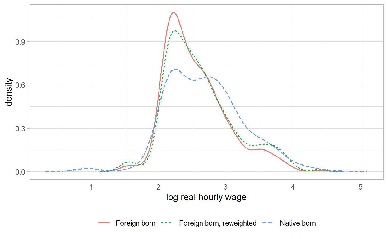
Figure 26.1: Observed log wage densities for native-born and foreign-born workers, and the counterfactual density of foreign-born wages reweighted to the native-born distribution of age, sex, and education. Reweighting closes part of the gap in the upper half of the distribution and almost none of it at the bottom.
26.3.2 RIF-Regression Decomposition
Reweighting gives an aggregate composition-structure split but not a detailed one: it cannot say how much of the ninetieth-percentile gap is due to education specifically. Firpo et al. (2009) supply the missing piece with the recentered influence function. For a distributional statistic \(\nu\), the RIF is a transformation of the outcome whose conditional expectation, projected on covariates, gives the effect of a marginal shift in the covariate distribution on \(\nu\). For the \(\tau\)-th quantile,
\[ \mathrm{RIF}(y; q_\tau) = q_\tau + \frac{\tau - \mathbf{1}\{y \le q_\tau\}}{f_Y(q_\tau)}, \]
where \(f_Y\) is the outcome density at the quantile. Replacing the outcome by its RIF and running an ordinary Oaxaca-Blinder decomposition then delivers a detailed decomposition of the quantile gap (Firpo et al. 2018).
rif_quantile <- function(y, tau) {
    q <- as.numeric(quantile(y, tau))
    f <- density(y, from = q, to = q, n = 1)$y
    q + (tau - as.numeric(y <= q)) / f
}

rif_decomp <- function(tau) {
    d <- ch
    d$rif <- NA_real_
    for (g in 0:1) {
        idx <- d$foreign.born == g
        d$rif[idx] <- rif_quantile(d$ln.real.wage[idx], tau)
    }
    mA <- colMeans(model.matrix(lm(reformulate(covs, "rif"),
                                   data = subset(d, foreign.born == 0))))
    mB <- colMeans(model.matrix(lm(reformulate(covs, "rif"),
                                   data = subset(d, foreign.born == 1))))
    bP <- coef(lm(reformulate(covs, "rif"), data = d))
    g  <- mean(d$rif[d$foreign.born == 0]) - mean(d$rif[d$foreign.born == 1])
    e  <- sum((mA - mB) * bP)
    c(quantile = tau, gap = g, explained = e, unexplained = g - e)
}

knitr::kable(
    round(t(sapply(c(0.1, 0.25, 0.5, 0.75, 0.9), rif_decomp)), 4),
    caption = paste("RIF-regression decomposition of the nativity log wage gap",
                    "at five quantiles. The gap is negligible at the tenth",
                    "percentile and large above the median, and the split",
                    "between characteristics and returns is far from constant",
                    "across the distribution.")
)| quantile | gap | explained | unexplained |
|---|---|---|---|
| 0.10 | 0.0017 | 0.0284 | -0.0267 |
| 0.25 | 0.0908 | 0.0373 | 0.0535 |
| 0.50 | 0.2389 | 0.0833 | 0.1557 |
| 0.75 | 0.2218 | 0.0924 | 0.1295 |
| 0.90 | 0.2892 | 0.1319 | 0.1573 |
The gap is essentially zero at the tenth percentile, about nine log points at the twenty-fifth, and between twenty-two and twenty-nine log points from the median upward. Characteristics account for roughly a third of the median gap and closer to half of the ninetieth-percentile gap, so the unexplained portion is largest in absolute terms at the top and largest as a share around the median. The tenth-percentile row is a reminder to read shares carefully: the explained component there exceeds a gap that is itself indistinguishable from zero, so the ratio is meaningless even though the levels are informative. A mean decomposition reports one number for a phenomenon that is not one phenomenon.
26.3.3 Counterfactual Distributions
Machado and Mata (2005) construct counterfactual distributions by simulating from a set of estimated conditional quantile regressions, integrating the group \(A\) conditional quantile process over the group \(B\) covariate distribution. Chernozhukov et al. (2013b) give the general theory, covering distribution regression as well as quantile regression, and provide functional inference: uniform confidence bands for the entire counterfactual distribution and formal tests of hypotheses such as stochastic dominance or no-effect-anywhere. That last capability matters, because a decomposition performed at five quantiles and interpreted as five separate findings has a multiplicity problem that a uniform band solves. The quantile and distributional methods chapter develops the estimation side of these tools.
26.4 Shapley Decompositions
Every decomposition considered so far has an ordering or reference ambiguity. The three-fold Oaxaca decomposition has an interaction term that must be assigned to one side or the other; the two-fold version needs a reference vector; a sequential specification table depends on the order of entry. Shorrocks (2013) observes that this is exactly the problem cooperative game theory solves, and that the Shapley value supplies the unique attribution satisfying efficiency (the parts sum to the whole), symmetry (identically contributing factors receive identical shares), and the null-player property.
The recipe: treat each factor as a player, define the worth of a coalition as the value of the statistic when only that coalition’s factors are active, and assign each factor its average marginal contribution over all orderings. The result is exact and order-free by construction.
The most common application is decomposing an \(R^2\) or an inequality index across groups of covariates.
groups <- list(age       = "age",
               gender    = "female",
               education = c("LTHS", "some.college", "college",
                             "advanced.degree"))

worth <- function(S) {
    if (!length(S)) return(0)
    summary(lm(reformulate(unlist(groups[S]), "ln.real.wage"),
               data = ch))$r.squared
}

all_subsets <- function(x)
    do.call(c, lapply(0:length(x), function(m) combn(x, m, simplify = FALSE)))

G <- names(groups); k <- length(G)
shapley <- setNames(numeric(k), G)
for (g in G) {
    for (S in all_subsets(setdiff(G, g))) {
        w <- factorial(length(S)) * factorial(k - length(S) - 1) / factorial(k)
        shapley[g] <- shapley[g] + w * (worth(c(S, g)) - worth(S))
    }
}

round(c(shapley, total = sum(shapley), full_R2 = worth(G)), 4)
#>       age    gender education     total   full_R2
#>    0.0404    0.0449    0.2125    0.2978    0.2978
The Shapley shares sum exactly to the full model’s \(R^2\), which is the efficiency property doing its work. Education accounts for roughly seventy percent of the explained variance and age and sex for the remainder in roughly equal shares, and these numbers do not depend on any ordering choice.
Two limitations. The computation is exponential in the number of factors, so grouping is necessary beyond about fifteen factors, and the grouping is itself a modeling choice. And a Shapley share of explained variance is a descriptive quantity: it says how much predictive content a factor group carries, not how much of a causal effect runs through it. The same caution that applies to variance-explained language everywhere applies here.
26.5 Variance Decompositions in Two-Way Models
A different decomposition question asks how much of the variance of an outcome is attributable to distinct sources of heterogeneity. The canonical case is Abowd et al. (1999)’s decomposition of log wages into worker effects, firm effects, and their covariance,
\[ y_{it} = \alpha_{i} + \psi_{J(i,t)} + x_{it}'\beta + \varepsilon_{it}, \qquad \mathrm{Var}(y) = \mathrm{Var}(\alpha) + \mathrm{Var}(\psi) + 2\,\mathrm{Cov}(\alpha, \psi) + \cdots, \]
where the covariance term is read as the degree of assortative matching between high-wage workers and high-wage firms. Early applications of this decomposition consistently found the covariance to be near zero or negative, which was puzzling: it suggested that good workers systematically sorted into bad firms.
M. J. Andrews et al. (2008) identified the explanation as limited mobility bias. The worker and firm effects are identified only from workers who move between firms, and when movers are scarce, both sets of effects are estimated with substantial error. The estimation errors in \(\hat\alpha\) and \(\hat\psi\) are mechanically negatively correlated, because a worker’s wage is split between the two, so the plug-in covariance is biased downward and the plug-in variances are biased upward. The following simulation generates data in which the true correlation between worker and firm effects is exactly zero.
library(fixest)

sim_akm <- function(nfirm = 150, nwork = 3000, movers_frac = 0.2, seed = 1) {
    set.seed(seed)
    psi   <- rnorm(nfirm)      # true firm effects
    alpha <- rnorm(nwork)      # true worker effects, independent of psi

    f1    <- sample(nfirm, nwork, replace = TRUE)
    mover <- runif(nwork) < movers_frac
    f2    <- ifelse(mover, sample(nfirm, nwork, replace = TRUE), f1)

    d   <- data.frame(w = rep(seq_len(nwork), 2), f = c(f1, f2))
    d$y <- alpha[d$w] + psi[d$f] + rnorm(nrow(d), 0, 0.5)

    fe <- fixef(feols(y ~ 1 | w + f, data = d))
    ah <- fe$w[as.character(d$w)]
    ph <- fe$f[as.character(d$f)]
    ok <- !is.na(ah) & !is.na(ph)

    c(var_firm = var(ph[ok]), cor_worker_firm = cor(ah[ok], ph[ok]))
}

shares <- c(0.05, 0.10, 0.20, 0.40, 0.80)
out    <- t(sapply(shares, function(m) sim_akm(movers_frac = m)))

knitr::kable(
    round(cbind(mover_share = shares, out), 3),
    caption = paste("Plug-in variance decomposition of a two-way fixed-effects",
                    "wage model when the true correlation between worker and",
                    "firm effects is zero. With few movers the estimated",
                    "correlation is strongly negative and the firm-effect",
                    "variance is inflated, an artifact of estimation error",
                    "rather than a feature of the labor market.")
)| mover_share | var_firm | cor_worker_firm |
|---|---|---|
| 0.05 | 1.971 | -0.576 |
| 0.10 | 1.066 | -0.217 |
| 0.20 | 0.886 | -0.058 |
| 0.40 | 0.845 | -0.032 |
| 0.80 | 0.854 | -0.019 |
With five percent of workers moving, the estimated correlation between worker and firm effects is strongly negative, and the firm-effect variance is more than double the value it settles at once mobility is high. Both distortions shrink as mobility rises, and the correlation approaches its true value of zero. A second problem lurks at the low-mobility end: when few workers move, the bipartite worker-firm network fragments into components that are not connected to each other, and effects in different components are identified only up to component-specific constants, which inflates the apparent variance further.
Kline et al. (2020) provide the modern solution. Their leave-out estimator constructs each variance component using, for every observation, an estimate of the fixed effects that excludes that observation, which removes the own-observation bias exactly in finite samples rather than asymptotically. The estimator is computationally demanding but has become the standard, and applied papers reporting AKM variance components without a leave-out or split-sample correction should be read as reporting upper bounds on variance and lower bounds on covariance.
The same lesson generalizes well beyond labor economics. Any variance decomposition whose components are themselves noisily estimated (teacher value-added, hospital quality, manager effects, store effects, physician effects) suffers the same bias, and the same corrections apply. The clustered inference and multilevel model chapters give the shrinkage-based alternatives that are appropriate when the goal is prediction of individual effects rather than estimation of their dispersion.
26.6 Decompositions of Estimators
A final family of decompositions takes an estimator rather than a gap as its object, and asks what weighted average of underlying comparisons it computes. The best-known instance is Goodman-Bacon (2021)’s result that the two-way fixed-effects difference-in-differences estimator is a variance-weighted average of all possible two-group two-period comparisons, including comparisons that use already-treated units as controls and can therefore receive negative weight. The staggered adoption section of the difference-in-differences chapter develops this at length.
The general principle is worth extracting, because it applies to many estimators beyond difference-in-differences. When an estimator can be written as a weighted average of elementary comparisons, computing and displaying those weights is a diagnostic that no amount of robustness checking substitutes for. Negative weights, weights concentrated on a handful of observations, or weights that load on comparisons the design was never meant to make are all failures that a coefficient and standard error conceal. The same decomposition logic has been applied to two-way fixed effects with continuous treatments, to instrumental variables estimators with multiple instruments, and to matching estimators, and in each case the finding is the same: the estimand is a weighted average whose weights are determined by the design and the data rather than by the researcher’s intent.
26.7 Practice
Decomposition results are unusually easy to report in ways that mislead, and unusually easy to fix.
State the counterfactual in words before reporting numbers. “How much of the gap would remain if foreign-born workers had native-born workers’ education” is a different question from “how much would the gap fall if we raised foreign-born workers’ education”, and the second is the policy question. Jackson and VanderWeele (2018)’s disparity-reduction framing is usually the one decision-makers want.
Report the reference-choice sensitivity. A single two-fold decomposition is one point in a range that the data do not narrow, and the range is often wide enough to change the conclusion.
Normalize categorical variables before reporting a detailed decomposition (Yun 2005), and report common support.
Use the conditional decomposition rather than a sequential specification table whenever the claim is about which covariates account for a coefficient movement (Gelbach 2016). It is exact, order-free, and comes with standard errors, and it frequently reveals offsetting contributions that the sequential table hides.
Go beyond the mean when the gap plausibly varies across the distribution, which is nearly always. The RIF decomposition costs a few lines of code and answers a question the mean decomposition cannot.
Correct variance decompositions for estimation error in the components, and do not interpret a negative estimated covariance between noisily estimated effects as evidence about the world.
Never label the unexplained component “discrimination”, “the treatment effect”, or “the mechanism”. It is the part of the gap that the included covariates and the assumed functional form do not account for, and it absorbs every specification error in the model.
26.7.1 Where This Shows Up in Practice
In labor economics and human resources analytics the decomposition is the standard tool for pay-equity analysis, and the reporting conventions above are not academic niceties: a pay-gap analysis submitted to a regulator or produced in litigation will be attacked precisely on reference choice, common support, and the omitted-variable content of the unexplained component. Presenting the sensitivity range preemptively is stronger than defending a single number.
In marketing and industrial organization the same arithmetic decomposes changes in market share, revenue, or customer lifetime value into price, mix, and volume components. The index-number problem is identical, and the standard practitioner habit of computing “price effect holding volume at last year” and “volume effect holding price at this year” is exactly the three-fold decomposition with the interaction term silently assigned. The Shapley approach resolves it, and for a two-factor or three-factor decomposition the computation is trivial.
In finance the conditional decomposition is the right tool for the ubiquitous question of which control set kills an anomaly. A paper reporting that a return premium survives industry adjustment but not size adjustment is making a claim about covariate contributions, and Gelbach (2016) converts it from a narrative about a specification table into an estimate with a standard error.
In public health and epidemiology the disparity-decomposition literature is the most developed application, and it is also where the causal framing has been worked out most carefully. The VanderWeele and Robinson (2014) treatment of race in regressions is required reading for anyone decomposing a gap defined by a non-manipulable characteristic, in any field.
26.8 Summary
Decomposition answers a different question from mediation. It splits an observed difference into accounting components rather than splitting a causal effect into pathways, and the arithmetic supplies no causal content on its own.
The Kitagawa-Oaxaca-Blinder decomposition splits a mean gap into parts due to differences in characteristics and parts due to differences in returns. It has two identification problems that no software default resolves: the reference coefficient vector is not determined by the data, and on the Chicago nativity gap the explained share ranges from fifteen to fifty-four percent depending on that choice; and the detailed decomposition of categorical variables is not invariant to the omitted category unless the coefficients are normalized.
Gelbach (2016)’s conditional decomposition solves the applied problem of attributing a coefficient movement to individual covariates. It is exact, order-invariant, and equipped with standard errors, and on the Chicago data it reveals that education more than fully accounts for the raw nativity penalty while age works in the opposite direction, a pattern a sequential specification table would have concealed.
Beyond the mean, reweighting constructs counterfactual distributions from a group-membership model alone, RIF regressions deliver detailed decompositions at any quantile, and counterfactual-distribution methods supply uniform inference over the whole distribution. On these data the nativity gap is indistinguishable from zero at the tenth percentile and twenty-nine log points at the ninetieth, and the split between characteristics and returns changes materially across the distribution.
Shapley decomposition resolves the ordering ambiguity that afflicts all of these methods, at exponential computational cost, and delivers the unique attribution satisfying efficiency and symmetry.
Variance decompositions in two-way fixed-effects models are biased when the effects are noisily estimated: with few movers, a simulation with zero true assortative matching produces a strongly negative estimated correlation and a doubled firm-effect variance. Leave-out estimation is the standard correction, and the lesson generalizes to every setting where a variance decomposition is built from estimated effects.